What is Descriptive Statistics? Statistical Notation

What is Descriptive Statistics?

Descriptive statistics is a branch of statistics that involves the collection, organization, and summary of data in a way that provides meaningful insights into the underlying data. It is used to describe the key features of a dataset, including measures of central tendency, measures of variability, and the distribution of data.

Statistics involves collecting, organising, analysing, interpreting and presenting data. You are familiar with the concept of statistics in daily life as reported in newspapers and the media, for example, baseball batting averages, airline on time arrival performance and economic statistics such as the Consumer Price Index (CPI). Statistical methods are essential to business analytics.

Microsoft Excel supports statistical analysis in two ways:

• With statistical functions that are entered in worksheet cells directly or embedded in formulas.
  
  
• With the Excel Analysis ToolPak add-in to perform more complex statistical computations.

A population consists of all items of interest for a particular decision or investigation—for example, all individuals in the United States of America who do not own cell phones, all subscribers to Netflix or all stockholders of Google.

A company such as Netflix keeps extensive records on its customers, making it easy to retrieve data about the entire population of customers. However, it would probably be impossible to identify all individuals who do not own cell phones.

A sample is a subset of a population. For example, a list of individuals who rented a comedy from Netflix in the past year would be a sample from the population of all customers. Whether this sample is representative of the population of customers — which depends on how the sample data is intended to be used — may be debatable; nevertheless, it is a sample.

Most populations, even the finite ones, are usually too large to practically or effectively deal with. For example, it would be unreasonable as well as costly to survey the TV viewers’ population of the United States of America. Sampling is also necessary when data must be obtained from destructive testing or from a continuous production process.

Thus, the process of sampling aims to obtain enough information to create a legal interpretation about a population. Market researchers, for example, use sampling to gauge consumer perceptions on new or existing goods and services, auditors use sampling to verify the accuracy of financial statements; and quality control analysts sample production output to verify quality levels and identify opportunities for improvement.

Descriptive statistics describes the data while inferential statistics infers about the population from the sample.

---

Understanding Statistical Notation

We typically label the elements of a dataset using subscripted variables, x1, x2, … and so on. In general, xi represents the ith observation. In statistics, it is common to use Greek letters such as σ(sigma), μ (mu) and π (pi), to represent the population measures and italic letters such as by (x-bar), s and p for sample statistics.

We will use N to represent the number of items in a population and n to represent the number of observations in a sample. Statistical formulas often contain a summation operator, (Greek capital sigma), which means that the terms that follow it are added together. Thus, understanding these conventions and mathematical notations will help you interpret and apply statistical formulas.

Central Tendency

Central tendency is the measurement of a single value that attempts to describe a set of data by identifying the central position within that set of data. Measurement of central tendency is also called as measures of central location. Some common terms used as valid measures of central tendency are as follows:

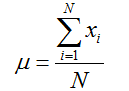
Mean: The mathematical average is called the mean (or the arithmetic mean), which is the sum of the observations divided by the total number of observations. The mean of a population is shown by the μ and the sample mean is denoted by x. If the population contains N observations x1 , x2 ,…, xN then, the population mean is calculated as

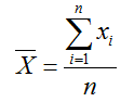
The sample mean of n sample observations x1, x2,…, xN is calculated as:

Median: The measure of location that specifies the middle value when the data is ordered (arranged from the least to the greatest or the greatest to the least) is the median. If the number of observations is odd, then the median is the exact middle of the sorted numbers, i.e., the 4 observations. If the number of observations is even, say 8, the median is the mean of the two middle numbers, i.e., mean of 4th and 5 th observation. We can use the Sort option of MS Excel to order the data as per the rank and then find the median. The Excel function MEDIAN (data range) could also be used. The median is meaningful for ratio, interval and ordinal data.

Mode: A third method of measuring the location is called mode. It is the observation/number/series that occurs the maximum number of times. The mode is valuable for datasets containing smaller number of unique values. You can easily identify the mode from a frequency distribution by identifying the value having the largest frequency or from a histogram by identifying the highest bar. You may also use the Excel function MODE.SNGL (data range). For frequency distributions or grouped data, the modal group is the group with the greatest frequency.

Midrange: A fourth measure of location that is used occasionally is the midrange. This is simply the average of the greatest and least values in the data set.

Variability

A commonly used measure of dispersion is the variance. Basically, variance is the squared deviations average of the observations from the mean. The bigger the variance is, the more is the spread of the observations from the mean. This indicates more variability in the observations. The formula used for calculating the variance is different for populations and samples. The formula for the variance of a population is:

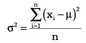
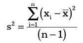
where xi is the value of the ith item, N is the number of items in the population and μ is the population mean. The variance of a sample is calculated by using the formula:

Consider an example of an organisation which kept records of its monthly sales figures of over two years, as shown in cells C3-C14 and F3-F14. The variance of the two years’ sales figures can be calculated in cell I4 of the spreadsheet by using the VAR.P function, as shown in Figure

Standard Deviation

The square root of the variance is the standard deviation. For a population, the standard deviation is computed as:

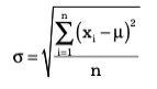
and for samples, it is

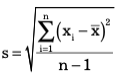
The standard deviation is usually easier to understand than the vari- ance because of similarity in its measure units that are same as the data units. Thus, it can be more easily related to the mean or other statistics measured in the same units.

The standard deviation is a popular measure of risk, particularly in financial analysis, because many people associate risk with volatility in stock prices. The standard deviation measures the tendency of a fund’s monthly returns to vary from their long-term average (as Fortune stated in one of its issues, “. . . standard deviation tells you what to expect in the way of dips and rolls. It tells you how scared you’ll be.”).

For example, a mutual fund’s return might have averaged 11% with a standard deviation of 10%. Thus, about two-thirds of the time the annualised monthly return was between 1% and 21%. By contrast, another fund’s average return might be 14% but have a standard devi- ation of 20%. Its returns would have fallen in a range of –6% to 34% and, therefore, is riskier.

Coefficient of Variation

The coefficient of variation (CV) provides a relative measure of the dispersion in data relative to the mean and is defined as:

CV = Standard Deviation / Mean

Often, the coefficient of variation is multiplied by 100 to be expressed as a percentage. This statistic is useful when comparing the variability of two or more data sets when their scales differ. The coefficient of variation offers a relative risk to return measure.

The smaller the coefficient of variation, the smaller the relative risk is for the return provided. The reciprocal of the coefficient of variation, called return to risk, is often used because it is easier to interpret.

That is, if the objective is to maximise return, a higher return-to-risk ratio is often considered better. A related measure in finance is the Sharpe ratio, which is the ratio of a fund’s excess returns (annualised total returns minus Treasury bill returns) to its standard deviation.

If several investment opportunities have the same mean but different variances, a rational (risk-averse) investor will select the one that has the smallest variance. This approach to formalising risk is the basis for modern portfolio theory, which seeks to construct minimum-variance portfolios.

Univariate, Bivariate and Multivariate Descriptive Statistics

In univariate descriptive statistics, only one variable deals with the information. Univariate data analysis is the simplest type of analysis. It is not concerned with causes or links and the primary goal of the analysis is to describe the data and identify patterns. Height is an example of univariate descriptive statistics.

In bivariate descriptive statistics, two variables are used for analysis. This sort of data analysis is concerned with causes and relationships and the goal is to determine the link between the two variables. Temperature and Hot Coffee sales in the winter season is the example of bivariate data.

In multivariate descriptive statistics, three or more variables are used for analysis. It is similar to bivariate, however there are more variables. The methods for analysing this data are determined by the objectives to be met. Regression analysis, path analysis, factor analy- sis and multivariate analysis of variance are some of the approaches. The description of these approaches are as follows:

• Multiple regression: The effects of many independent variables (predictors) on the values of predictor variables or outcome, are investigated in multiple regression analysis, also known as regression analysis. To evaluate the influence of each predictor on the dependent variable, regression determines a coefficient for each independent variable as well as its statistical significance, while holding other predictors constant.
  
  Regression analysis is frequently used by economists and other social scientists to investigate social and economic phenomena. Examining the influence of education, experience, gender and ethnicity on income is an example of a regression analysis.
  
  
  
• Factor analysis: When a study design has a large number of variables, it is generally beneficial to minimise the variables to a smaller number of components. There is no dependent variable with this strategy, hence it is called independence. Rather, the researcher is seeking for the data matrix’s underlying structure.
  
  A researcher uses factor analysis to reduce a huge number of variables to a smaller, more manageable number of components. Factor analysis identifies patterns among variables and groups closely related variables into factors. In survey research, one of the most popular applications of factor analysis is to examine if a large list of questions can be broken down into smaller groups.
  
  
  
  
• Path analysis: This is a graphical method of multivariate statistical analysis in which route diagrams represent the correlations between variables, as well as their orientations and the “paths” along which these associations move. Path coefficients are calculated by statistical software tools and their values represent the strength of links among variables in a researcher’s hypothesised model.
  
  
  
• Multiple Analysis of Variance (MANOVA): It is a more complicated version of the simpler analysis of variance, or ANOVA. MANOVA is a technique that allows researchers to adjust for correlations between two or more dependent variables in studies containing two or more of them.
  
  A study of health among three groups of teenagers: those who exercise frequently, those who exercise on occasion and those who never exercise is an example of a study for which MANOVA might be an acceptable approach. Multiple health-related outcome measures such as weight, heart rate and respiration rate would be possible with a MANOVA in this study.