
What is Sigma Level?
Sigma level is a statistical metric that is used for measuring the number of errors or defects in a process. The Sigma level indicates how the process varies from being perfect. This measurement is based on the Defects Per Million Opportunities (DPMO) parameter.
The Sigma level measures the process efficiency in the long term which also includes a potential 1.5 Sigma shift. This shift generally occurs over long periods. The 1.5 Sigma shift is considered to be an industry-wide standard estimate for measuring the Sigma levels of processes. This standard was originally devised by Motorola and later on, it was adopted throughout industries.
Table of Content
Characteristics of Sigma Level
The characteristics of Sigma level are as follows:
- The Sigma level is determined during the first phase of the DMAIC process, i.e. the Measure phase.
- The Sigma-level measurements can also be used throughout the DMAIC process.
- The Sigma level can be used for comparing the overall performance of an organization against the overall performance of other organizations.
- The Sigma level can be used for comparing the performance of a particular process of an organization against the performance of the organization’s other processes.
- The Sigma level can be used to determine the baseline performance of an organization or a specific process before making interventions for improvement actions.
- The Sigma level can be used to analyze the impact of improvement interventions on the performance of a process.
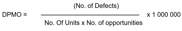
DPMO Formula
The Sigma level can be calculated using the following steps:
- Determine the total count of units produced.
- Measure the number of defect opportunities per unit.
- Count the number of defects.
- Determine the DPMO with the formula.
- The process Sigma can be calculated from the DPMO Sigma Conversion Table available freely.
Defects Per Opportunity (DPO)
A metric routinely used in Six Sigma is Defects Per Opportunity (DPO). The total number of defects, which are possible in a sample, is determined using the DPO metric which is calculated by the following formula:
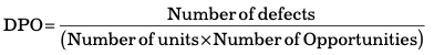
The number of characteristics of a product, which are used to test units in a sample, is the number of opportunities. For example, a piece of cloth may be measured in three units including length, width, and weight. In this case, the number of opportunities is 3. Assume that the total number of defects is 20 and the total number of units is 200; in this case, DPO = 20 / (200 *3) = 0.03 or 3 %
The value 0.03 shows that each of the 3 opportunities’ length, width, and weight has an average of 0.03 or 3 % defects in each unit. DPO is an indication of the probability of a process producing units free from defects.
Defects Per Million Opportunities (DPMO)
The DPO metric is used to calculate another Six Sigma metric called Defects Per Million Opportunities (DPMO) which indicates how many defects can a sample possibly have per million opportunities.
DPMO=DPO*1000000
Continuing our earlier illustration, DPMO would be = 0.03 * 1000000 = 30,000
DPMO 30,000 indicates that the business process is estimated to have 30,000 defects per million opportunities. The Defects Per Million Opportunities (DPMO) metric is useful in assessing the performance of an organization in terms of the quality of its products and/or services. The DPMO value is important in determining the process’s effectiveness.
A product that fails to meet the expectations of a customer due to some shortcomings in its product features is said to have a defect. Most of the time, defects get identified before the product is launched in the market. However, in some instances, defective products may reach the customer who may then either return them or lodge a complaint with the producer organization.
Based on the number of complaints registered and the defective products identified, the organization can then compare the available options for production and choose the best possible option that seems to produce the least number of defects. Redesigning the process to have the least number of variations may also be considered by the organization.
For correcting a defective process the root cause analysis should be carried out to determine all possible causes of defects and classify defects as per their frequency and the likelihood of occurrence. The defects that occur rarely can be overlooked to save resources and time. The more frequently occurring defects need to be analyzed and the production process should be corrected accordingly.
Assume that P represents the number of deviations that arise during the manufacturing process. If this P is divided by the total number of units produced, we will obtain defects per unit. In this case, the total number of units that are free of defects will give the yield. The Poisson distribution ratio in this case would give the probability of getting any number of deviations from good results.
A reference table called the Z table can be made use of to make such calculations. Once DPO is obtained, DPMO can be determined which would indicate how perfect the process of production is. DPMO is obtained by multiplying DPO by 1,000,000. The percentage of defects and yield forms important information. One can also conclude the yield and the Sigma conversion table once the DPMO percentage is known.
A value of more than 3.4 defects per million opportunities is not a Six Sigma level of perfection. This information is useful in the measuring stage of the Six Sigma process as it helps take decisions on what kind of adjustments and alterations in the process will be required or those that may be unnecessary.
Further, it also aids in controlling costs in the production process by bringing down the reasons for poor quality and repetition of tasks that are needed to produce a product as per customer expectations. However, one drawback of the Six Sigma DPMO determination is that this metric may be of great utility for large-scale production organizations but for organizations with smaller amounts of production, it may not be of much use.
Process Capability and Sigma Level
Quality and improvement initiatives in an organization are largely dependent on two important methodologies, namely Process Capability Analysis (PCA) and Six Sigma. In the process of manufacturing, quality, and process improvement, PCA emerges as a basic technique that is applied to achieve higher levels of customer satisfaction by bringing improvements in products, processes, and services. Process Capability Indices (PCIs) are the measures of process capability and the numeric values that represent the PCA.
The four most common measures of process capability are Cp, Cpk (Cpl, Cpu), and Cpm.
Cp is a process capability measure for the overall capability of the process. It is calculated as the ratio of the difference between the specification limits to the observed process variation. If Cp is greater than or equal to 1, it indicates a capable processor, and a value of Cp less than 1 indicates that the process is variable.
Cpu and Cpl are measures to determine whether or not the process variability is symmetric or not. It is calculated using the distance between the process mean and the upper specification limit (Cpu) or the lower specification limit (Cpl).
Cpk is the process capability related to both dispersion and centeredness. It is calculated as the minimum of Cpu and Cpl. If only one specification limit is provided, the Cpk value is calculated unilaterally.
The Cpm is a process capability index relating to capability sigma and the difference between the process mean and the target value.
The Six Sigma methodology helps an organization reduce process variation and facilitates augmentation of the organizational process capability. PCA is defined as the proportion of the spread of the actual process to the process spread that is allowed. This process spread is measured by six process standard deviation units. In a process capability study, the number of standard deviations that exist between the process mean and the nearest specification limits are stated in sigma units, similar to the Six Sigma methodology.
The capability of a process to perform as per specifications is expressed by the sigma quality level. A process is a combined use of methods and input resources such as equipment, materials, and people that work in harmony to produce a measurable output. There are inherent statistical variabilities in every process that may be determined, analyzed, and reduced to a certain extent using statistical techniques and methods.
Organizations should always consider the extent and the source of variability and make efforts to improve quality to decrease the variance in their production processes as much as possible. The extent of variability is inversely proportional to the quality and customer satisfaction. Thus, the critical-to-quality characteristics (CTQs) variability is a representation of the output uniformity. A large amount of variability indicates a large number of product non-conformances.
Process capability reflects the uniformity of a process. Variability in a process can arise in two forms. One is the inherent variability in a CTQ at a given time, and the second is the variability that arises in a CTQ over some time. It is important to remember that PCA measures CTQs, i.e. the functional parameters of a product and not the process itself.
Process capability draws a comparison between the output of an in-control state process to the limits specified by the PCIs. In other words, a process that is determined to be capable has most measurements within specification limits.
In the case of a direct process observation or a true process capability study, it is possible to draw inferences about process stability over some time by directly monitoring and also controlling the data collection methodology and understanding the time sequence of the data.
In the absence of direct observation of the process, the study is called a product characterization study where only sample units of the product are known. According to Montgomery (2009), in a product characterization study, the distribution of the product quality characteristic or the fraction that conforms to specifications, which is referred to as process yield, can only be estimated, notably, information about the stability or dynamic behavior of the process cannot be given.
There may be many statistical techniques involved in a PCA throughout the product cycle. Mostly PCA is made use of in development activities that take place before the manufacturing process, to quantify process variability. PCA is used to analyze this process variability with the specifications. PCA also helps in reducing or eliminating process variability.
PCA has nowadays become widely adopted as a measure of performance. PCA is generally determined from a sample of data obtained from a process and it helps in determining DPMO, capability indices, and the sigma quality level at which the process operates. It is usual to incorporate the Six Sigma spread in the distribution of quality characteristics of a product to measure the process capability.
For a process with a quality characteristic having a normal distribution with a process mean µ and the process standard deviation σ, the Lower Natural Tolerance Limit is LNTL = µ – 3σ, and the Upper Natural Tolerance Limit is UNTL = µ+ 3σ.
A point to be noted here is that the natural tolerance limits of a process shall include 99.73% of the variable, and the remaining 0.27% of the process output shall be located outside the natural tolerance limits.
Statistical Techniques of Sigma Level
For carrying out PCA, the following statistical techniques can be used:
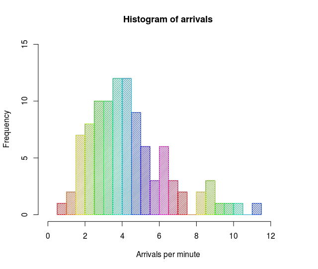
Histograms
A histogram is a graphical display of frequencies in statistics. A histogram is one of the seven basic tools of quality assessment and also finds great use in determining the process capability. It is a great tool for visualizing process performance.
It is possible to use histograms to immediately determine the reason for the poor performance of a process. It is generally assumed that quality characteristics are likely to have a normal distribution, thus a histogram with information on the sample mean and sample standard deviation can be of great value to obtain information about the process capability.
A normality assumption in such cases can be made by the visual appearance of the histogram. In the case of a skewed histogram, the estimate of the process capability may be inaccurate. There are also some disadvantages to using histograms. Division of the range of a variable into classes is a fundamental necessity. But a histogram may not be of much use for small samples as it may require a fairly large number of moderately stable observations.
Probability Plots
A probability plot can also be used to evaluate and determine the parameters of a distribution, such as a shape, median, i.e., center, and variability, i.e. the spread. In the case of probability plots, the division of the range of variables into class intervals may be unnecessary. An important advantage of probability plots is that they can be used for relatively smaller samples.
However, the characteristics and quality of the data affect the inferences drawn on process capability. A disadvantage of probability plots is that they are not objective procedures even though normal probability plots are very useful in process capability studies. The fat pencil test is used in cases where a normal probability plot is used, to test the adequacy of the normality assumption.
Once data is plotted against a theoretical normal distribution, the points so plotted should form an approximate straight line. If the data points are not placed in a straight line, it is considered a deviation from normality. In this way, the fat pencil test is performed.
Design of Experiments (DOE)
Critical parameters associated with a process can be determined using a DOE. For an enhanced capability and performance of a process, optimal settings of parameters are required which may be determined by a DOE. The controllable input variables in a process can be varied and the effects of these process variables on the output or response can be analyzed by a DOE.
It also helps managers isolate the influential process variables and determine the levels of these variables to optimize process performance. One of the important uses of DOE is to identify and estimate the sources of variability in a process. The tool has been widely adopted in the manufacturing industry even for the resolution of more general problems rather than merely estimating the process capability.
Control Charts
This is a useful tool for establishing a baseline for the process capability or process performance. An important use of a control chart is as a monitoring device that can demonstrate the effects of changes in a process on the process performance. The principle function of a control chart is to determine whether a manufacturing or business process is under statistical control or not. This chart also demonstrates systematic patterns in process output.
Further, a control chart is used before using PCIs as at this time the process needs to be in a state of statistical control. If a process seems to be in a state of statistical control in a control chart, it can be used with a reasonable degree of surety and predict the future performance of the process.
However, if a control chart indicates that the process under observation is not in statistical control, the source of variation can be determined from the pattern revealed by the control chart. And it can then be eliminated to achieve process control.
Most importantly, the control chart helps separate the signal (a real problem) from noise (natural process variability). This feature is the key to effective process control and improvement. Control charts should be considered as a primary technique of PCA where both variables and attributes control charts can be used.
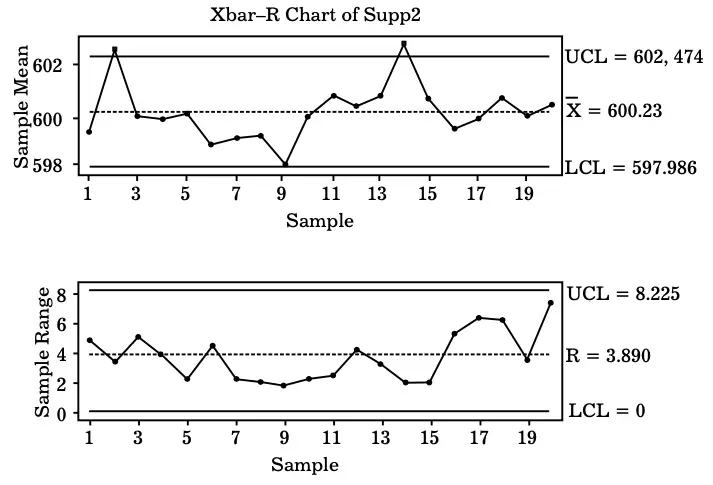
Sample Control Chart
Throughput Yield and Sigma Level
Throughput yield is also a Six Sigma metric that is used routinely. This metric indicates the process’s ability to produce units or products that are free of any defects. The throughput Yield (Yt) is calculated by using the Defects per Unit (DPU).
The classic Yield metric considers only the number of defective units in contrast to the Throughput Yield which takes into consideration the total number of defects occurring on those units. Further, the classic yield metric takes into account only the defects that get passed to a customer leaving out the reworked defects which are a source of internal waste.
Throughput Yield holds an important place in the Six Sigma study because it measures the efficiency of a process. An important advantage of this metric is that it is a universal standard metric. It finds applicability in processes of any nature thereby enabling the comparison of different processes on a level ground.
Throughput Yield helps in determining the inherent ability of a process to meet the stated specifications. Alternately, it determines the ability of a process to produce units without defects. The calculation of Yield leads the way to the calculation of Throughput Yield. Yield is determined by the ratio of the number of units that are acceptable and the number of units that enter the production process.
As can be seen in the formula, the number of acceptable units throws no light on how many units were reworked. Thus, it is not a true measure.
Therefore, another metric, First Pass Yield, was introduced.
However, even this metric lacked perfection. As you can see, both the above metrics use defective units as their basis for measurement. However, there are chances of more than one defect occurring in a single defective unit. Unless this inherent drawback is eliminated, Yield or First Pass Yield cannot be considered a true measure of the efficiency of the product.
Throughput Yield calculation is based on the number of defects and uses DPU (defects per unit) for its calculation. DPU is calculated by using the following formula.
and
Thus, Throughput Yield can be used effectively to measure the success rate of a process.
There can be multiple sub-processes that exist together to deliver the final product. These processes may be placed consecutively one after the other in a row or may even operate side by side to deliver output to a common single process. A concept called Rolled Throughput Yield (RTY) is used to determine the overall Throughput Yield.
There is a slight difference in the formula for calculating Rolled Throughput Yield (RTY) of a parallel process and a serial process.
- RTY for a serial process is determined by first measuring the TPY of all sub-processes and then multiplying these TPYs.
- RTY for a parallel process is calculated as the minimum value of all the individual processes operating parallel to each other.
Business Ethics
(Click on Topic to Read)
- What is Ethics?
- What is Business Ethics?
- Values, Norms, Beliefs and Standards in Business Ethics
- Indian Ethos in Management
- Ethical Issues in Marketing
- Ethical Issues in HRM
- Ethical Issues in IT
- Ethical Issues in Production and Operations Management
- Ethical Issues in Finance and Accounting
- What is Corporate Governance?
- What is Ownership Concentration?
- What is Ownership Composition?
- Types of Companies in India
- Internal Corporate Governance
- External Corporate Governance
- Corporate Governance in India
- What is Enterprise Risk Management (ERM)?
- What is Assessment of Risk?
- What is Risk Register?
- Risk Management Committee
Corporate social responsibility (CSR)
Lean Six Sigma
- Project Decomposition in Six Sigma
- Critical to Quality (CTQ) Six Sigma
- Process Mapping Six Sigma
- Flowchart and SIPOC
- Gage Repeatability and Reproducibility
- Statistical Diagram
- Lean Techniques for Optimisation Flow
- Failure Modes and Effects Analysis (FMEA)
- What is Process Audits?
- Six Sigma Implementation at Ford
- IBM Uses Six Sigma to Drive Behaviour Change
Research Methodology
Management
Operations Research
Operation Management
- What is Strategy?
- What is Operations Strategy?
- Operations Competitive Dimensions
- Operations Strategy Formulation Process
- What is Strategic Fit?
- Strategic Design Process
- Focused Operations Strategy
- Corporate Level Strategy
- Expansion Strategies
- Stability Strategies
- Retrenchment Strategies
- Competitive Advantage
- Strategic Choice and Strategic Alternatives
- What is Production Process?
- What is Process Technology?
- What is Process Improvement?
- Strategic Capacity Management
- Production and Logistics Strategy
- Taxonomy of Supply Chain Strategies
- Factors Considered in Supply Chain Planning
- Operational and Strategic Issues in Global Logistics
- Logistics Outsourcing Strategy
- What is Supply Chain Mapping?
- Supply Chain Process Restructuring
- Points of Differentiation
- Re-engineering Improvement in SCM
- What is Supply Chain Drivers?
- Supply Chain Operations Reference (SCOR) Model
- Customer Service and Cost Trade Off
- Internal and External Performance Measures
- Linking Supply Chain and Business Performance
- Netflix’s Niche Focused Strategy
- Disney and Pixar Merger
- Process Planning at Mcdonald’s
Service Operations Management
Procurement Management
- What is Procurement Management?
- Procurement Negotiation
- Types of Requisition
- RFX in Procurement
- What is Purchasing Cycle?
- Vendor Managed Inventory
- Internal Conflict During Purchasing Operation
- Spend Analysis in Procurement
- Sourcing in Procurement
- Supplier Evaluation and Selection in Procurement
- Blacklisting of Suppliers in Procurement
- Total Cost of Ownership in Procurement
- Incoterms in Procurement
- Documents Used in International Procurement
- Transportation and Logistics Strategy
- What is Capital Equipment?
- Procurement Process of Capital Equipment
- Acquisition of Technology in Procurement
- What is E-Procurement?
- E-marketplace and Online Catalogues
- Fixed Price and Cost Reimbursement Contracts
- Contract Cancellation in Procurement
- Ethics in Procurement
- Legal Aspects of Procurement
- Global Sourcing in Procurement
- Intermediaries and Countertrade in Procurement
Strategic Management
- What is Strategic Management?
- What is Value Chain Analysis?
- Mission Statement
- Business Level Strategy
- What is SWOT Analysis?
- What is Competitive Advantage?
- What is Vision?
- What is Ansoff Matrix?
- Prahalad and Gary Hammel
- Strategic Management In Global Environment
- Competitor Analysis Framework
- Competitive Rivalry Analysis
- Competitive Dynamics
- What is Competitive Rivalry?
- Five Competitive Forces That Shape Strategy
- What is PESTLE Analysis?
- Fragmentation and Consolidation Of Industries
- What is Technology Life Cycle?
- What is Diversification Strategy?
- What is Corporate Restructuring Strategy?
- Resources and Capabilities of Organization
- Role of Leaders In Functional-Level Strategic Management
- Functional Structure In Functional Level Strategy Formulation
- Information And Control System
- What is Strategy Gap Analysis?
- Issues In Strategy Implementation
- Matrix Organizational Structure
- What is Strategic Management Process?
Supply Chain

