Methods of Sales Forecasting

What is Sales Forecasting?

Sales forecasting is the process of predicting future sales performance based on historical data, market trends, and other relevant factors. It is an essential activity for businesses of all sizes, as it helps them plan and make informed decisions about their operations, including production, inventory management, and marketing.

Criteria for Adopting a Forecasting Method

Several methods of sales forecasting are available, and the management can choose the one that will work best for them depending on the following criteria.

• Simplicity: The forecaster should choose a method that is simple and easily understood by the executives.
  
  
• Credibility: Forecasters should choose methods they understand well and know are reliable. This is important to interpret the results of the method and increase accuracy.
  
  
• Economy: The importance of the forecast should justify the cost of the method. If the forecast is very important, it makes sense to choose an expensive method that gives high levels of accuracy; otherwise, the adopted method should be of low cost.
  
  
• Availability: The forecasting method should be able to make meaningful results quickly available. A method that takes too long to produce results does not help managerial decisions.

One must remember that predicting anything in the future, including sales, is often inaccurate, so one must choose a method of forecasting and improve it such that the forecast is as realistic as possible. A good sales forecasting technique minimises the departure of the actual sales from the forecast.

---

Methods of Sales Forecasting

Forecasting methods can be of two types:

• Qualitative forecasting methods
• Quantitative forecasting methods

Qualitative forecasting methods are based on opinions and intuition, whereas quantitative forecasting methods use mathematical models and relevant historical data to generate a forecast. The table below summarises the differences between the two approaches:

Qualitative methods	Quantitative methods
Relevant in situations where little to no information exists	Relevant in situations where historical data exists
Useful for new products and new technology	Useful for existing products and technology
Involves human judgement, intuition and experience	Involves mathematical techniques
Their strength is to include the latest changes and access to inside information	Their strength is objectivity, consistency and ability to handle huge quantities of data
Limited by being prone to personal bias	Limited by their dependence on data

Qualitative Methods

Qualitative forecasting methods are based on human factors, such as opinions and intuition. In this section, we will discuss some of the most widely used methods.

User Expectations

In this method, the business approaches its customers directly to determine their requirements in the near future. The business asks its customers about the quantity and quality of the goods they will purchase, when and where they will buy, etc.

The user expectation method is appropriate for industrial products such as raw materials, machinery, and other items used for industrial purpose. This is because the number of buyers is limited for industrial products unlike consumer goods where each customer accounts for a very small quantity. Thus, industrial products can be surveyed exhaustively.

The user expectations method has the following advantages:

• The information is obtained directly from the customer.
  
  
• This method is highly suitable in the case of industrial goods where the number of customers is few.

The user expectations method has the following limitations:

• There is a chance that the expectations of the buyer may change in future.
  
• It works only for short-term forecasting.
  
  
• It does not work for making forecasts regarding consumer goods.

Sales Force Composite

In the sales force composite method, salespersons are approached for their opinion regarding the sales trends in their respective territories, and these opinions are consolidated to build the overall sales forecast. The sales personnel provides the estimates of the sales of a product or service in a particular sales territory, during a given period.

This method is the bottom-up approach wherein the sales force offers their opinion on sales trends to the top management. The strength of this method comes from the fact that salespersons have a good understanding of their sales territories and customers.

The weakness of this method is that it is prone to the personal bias of the salespersons. Moreover, salespersons may not know how to use economic and statistical indicators correctly. They might only consider the microeconomic factors and neglect the macroeconomic environment. This problem can be somewhat remedied by training the sales force in forecasting techniques.

Jury of Executive Opinion

The jury of executive opinion is a widely used qualitative method of sales forecasting. The opinions of a small group of top-level managers and executives from different departments, such as sales, finance, marketing and production are collected and used to predict sales for a given period.

This method is usually employed when the issue is complex as the top-level executives have years of experience in their field and a deep understanding of the organisation’s strengths and weaknesses and the risk factors and opportunities in the relevant industry.

They also better understand the macroeconomic factors that can influence the sales trend. In the jury of executive opinion, the group of top-level managers and executives uses its managerial experience, and sometimes also includes the results of statistical models.

This method includes judgement and other soft human factors, such as personal opinions and intuition to make predictions. The jury of executive opinion method can be of two types: the top jury method and percolated jury method. In the top jury method, only the top executives can participate and in the percolated jury method, a large number of marketing sales executives participate.

Delphi Technique

The Delphi method is a method of choice when a long-term forecast is needed on complex issues where expert opinion is the only available source of information. The Delphi method works on the assumption that the combined knowledge of a panel of experts will generate a forecast at least as good (and most likely better) as the one generated by a single member.

In this method, a panel of members with expertise in the given area are approached with a questionnaire and their feedbacks are organised into a summary. If any expert’s answer deviates too much from the median, they offer an explanation that is added to the summary.

The updated summary is sent to all the panel members again. They review the summary and if they think necessary, they can reconsider or revise their forecast given the feedback of other members. The limitation of the Delphi method is that it can be a time-consuming process, especially if there is not much consensus between panel members initially.

The steps in the Delphi method are given below:

• A questionnaire is sent to a panel of experts, either internal or external to the organisation, to obtain their independent estimates of future sales.
  
  
• The independent estimates are organised in the summary and the summary report is submitted to panel members for review.
  
  
• Experts can review the estimates made by other experts and if they think necessary, they may reconsider or revise their estimates.
  
  
• The process is repeated for multiple round still the panel reaches a consensus on the forecast.

Market Test

In the market test method, a sales forecast is made based on the outcome of a direct market test. It is used more commonly by consumer goods marketers. When used by industrial goods marketers, this method is called a market probe. The market test helps to make sales forecasts for new product launches.

It helps the firm decide if the market will accept the product or not. In the market test method, the new product is first introduced in selected geographical areas that are representative of the final market to estimate the product’s acceptance and demand in the selected areas.

Based on the customer response, the firm can forecast the sales of the product and decide whether commercialisation is a viable option or not. The market test is a quite reliable method, but care must be taken to select areas that truly represent the overall market.

Hyderabad, a city in India is proved to a successful test market for various major brands. Lipton Ice tea, Kinley Water by Coca-Cola, Nizoral anti-dandruff shampoo all were tested in this city. One of the major reasons Hyderabad being suitable for test marketing is because IT hub people from all across the region come here therefore it represents a national market.

Despite being valuable as a sales forecasting tool, it is limited by the fact that it is a time-consuming process since the results can only be reliable if the test is carried out for a sufficient amount of time. It takes significant time to deliver results, during which market conditions may change and the results may not be a true representation of the whole market.

Quantitative Methods

Quantitative methods for sales forecasting are different from qualitative methods as they make use of mathematical tools and historical data. These methods are more objective than qualitative methods and usually more time and cost-effective. Let us discuss the widely used quantitative methods in the sections below:

Time Series Analysis

Time-series analysis is one of the most widely used methods for the prediction of long-term forecasting. The term time series refers to a sequential order of values of a given variable at equal time intervals. A time-series depicts the relationship between two variables, one being time and the other any measurable variable. The quantified variable may show an increase or decrease with reference to time.

Time series analysis explains the reason behind the values observed at different points in time. A time-series model aims to identify patterns in historical data and extrapolate them into forecasts.

A time series is generated by collecting a series of information over given points in time. For example, the number of mobile phones sold in January can be used as a time series. There are 31 days in January and if the sales per day are recorded and arranged in ascending order, it will generate the following series:

Date	Number of Units Sold
January 1	28
January 2	35
January 3	32
…..	…..
January 31	23

Time series data, such as the one above can be applied to a time series forecasting model to make predictions, such as estimating the sales for February.

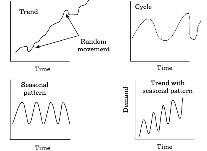
A time-series problem has the following time-based key components:

• Level: Level is the average or baseline value in the time series.
  
  
• Trend: Trend is the long-term increase or decrease in the values of the target variable with time. A trend can be upward, downward, or horizontal (no trend). It can be linear or exponential.
  
  
• Cycles: This component accounts for the recurring pattern of data above and below the trend line. This component exists when the data shows inclines or declines that are not of a fixed period. Cycles differ from seasonal patterns because the average length of cycles is longer (usually, more than one year).
  
  
• Seasonality: Seasonality exists when there is a tendency of patterns to repeat at regular intervals.
  
  
• Irregularity/Noise: This component exists when there are random variations that can occur in the data that cannot be explained through trends, cycles, or seasonality. It accounts for short-term, unexpected and non-recurring factors that influence the time series data.

Three factors are important in time series analysis and forecasting:

• Autocorrelation: Autocorrelation is the degree of correlation of a time series with its past values, i.e., the tendency of data patterns to repeat themselves.
  
  
• Seasonality: Seasonality is a measure of how often observations and patterns repeat themselves at regular intervals.
  
  
• Stationarity: Stationarity is the property of the mean, variance and an autocorrelation structure to remain the same over time.

The time series analysis is quite useful when there is sufficient past data of a reliable nature is available. It helps to understand the rate of growth, the extent and the direction of periodic fluctuations when conditions are relatively stable.

Moving Average

Long-term forecasting of sales trends can also be done using the moving average or rolling mean method. The moving averages method examines the underlying pattern of a set of data to provide an estimate of future values. The moving averages method uses time-series data to smooth out random, short-term fluctuations in the data set by creating a constantly updated average. The technique generates an average of a set of numbers in a given range whilst moving the range.

In other words, a rolling mean is calculated by adding the values of the observations of the last ‘n’ period and then dividing that number by ‘n’ to get an average. This mean is now considered the forecast for the next period. From the perspective of sales, using the moving averages method, the sales forecasting is attained by taking average of past sales over a desired number of past periods (which can be years, months or weeks).

Extending the moving average to include more periods may increase the smoothening effect but reduces the sensitivity of forecast. Long periods provide too many opportunities for significant changes to occur in demand pattern. To reduce this risk, organisations can base its forecast on the average demand during short periods say three months.

Like an average, a moving average also represents the middle value of a set of numbers, but the average is calculated several times for several subsets of data. For instance, if a two-year moving average is to be calculated for a data set from 2002, 2003, 2004 and 2005, the averages for the subsets 2002/2003, 2003/2004 and 2004/2005 will be calculated. Moving averages are usually plotted and are best visualised.

The moving averages method can have the following variations:

• Simple moving average (SMA): SMA is an equally weighted mean of n records. The formula for SMA is:
  
  Simple Moving Average = (A1 + A2 +……+ An)/n
  
  where Ai is the data point in the ith period.
  
  
• Weighted moving average (WMA): WMAassigns more weight to recent data points and less weight to older data points. It is calculated by multiplying each observation in the data set by a predetermined weighting factor. The formula for WMA is:
  
  Weightage Moving Average= (A1* W1+A2*W2+……+ An* Wn)
  
  where Ai is the data point in the ith period and Wi its predetermined weighting factor.where Ai is the data point in the ith period and Wi its predetermined weighting factor.
  
  
• Exponential moving average (EMA): EMA is also a weighted average where more weight is given to the data observed in more recent times than older data. But here the weighting factors decrease exponentially. The formula for the EMA is:
  
  Exponential Moving Average=(C – P) *(2/(n+1))+P
  
  where C is the current data point and P is an exponential moving average of the previous period (simple average used for the first period).

Since both WMA and EMA assign more weight to recent observations,they are more responsive to changes.

Let us discuss the application of the moving averages method with the help of an example.

Example: Let us calculate the five year moving average from the following data set:

Year	Sales (in lakhs)
2003	8
2004	12
2005	10
2006	16
2007	18
2008	10
2009	8
2010	6
2011	14
2012	16

The mean (average) sales for the first five years (2003-2007) will be calculated by finding the mean from the first five years (i.e. adding the five sales totals and dividing by 5). This will give the moving average for 2005 (the center year) = 12.8 Lakhs [(8 Lakhs + 12 Lakhs + 10 Lakhs + 16 Lakhs + 18 Lakhs)/5]

The average sales for the second subset of five years (2004 – 2008), centered around 2006, is 13.2 Lakhs [(12 Lakhs + 10 Lakhs + 16 Lakhs + 18 Lakhs + 10 Lakhs)/5]

The average sales for the third subset of five years (2005 – 2009), centered around 2007, is 12.4 Lakhs [(10 Lakhs + 16 Lakhs + 18 Lakhs + 10 Lakhs + 8 Lakhs)/5]

The calculation will continue for each five-year average, until the end of the set (2009-2013) is reached. This will give a series of points (averages) that can be used to plot a chart of moving averages (that is done using Microsoft Excel in most of the cases).

Regression & Correlation

Correlation is the degree to which two or more variables are related. Correlation analysis is done using various statistical tools and techniques to determine the degree of correlation between two or more variables. Correlation analysis helps to quantify the relationship between two or more variables.

For sales forecasting, two factors are also correlated.

For example, daily sales of ice cream can be correlated with the daily maximum temperature. Similarly, the sales of a specific product can be correlated with promotional expenditure, advertising expenditure and the efficiency of the sales force. Correlation analysis estimates a sample correlation coefficient, denoted r, that ranges between -1 and +1. The correlation between two variables can either be positive (i.e., higher levels of one variable correlate to higher levels of the other) or negative (i.e., higher levels of one variable correlate to lower levels of the other).

The sign of r indicates the direction of the association, while the magnitude of the r indicates the strength of the association. For instance, a correlation of r = 0.9 indicates a strong and positive relationship between the two variables whilst a correlation of r = -0.4 indicates a weak and negative relation. r ~ 0 shows that there is no linear relationship amongst two continuous variables.

Let X and Y be the two random variables, then the population correlation coefficient σ_XY between X and Y is given by the formula:

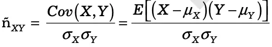
ñ X Y

Where:

ρ_XY = Population correlation coefficient between X and Y

Cov = Covariance

E = Expected value operator

μ_X = Mean of the variable X

μ_Y = Mean of the variable Y

σ_X = Standard deviation of X

σ_Y = Standard deviation of Y

Correlation can be represented using graphs, such as the one shown in Figure below that shows four hypothetical scenarios where one continuous variable is plotted along the X-axis and the other along the Y-axis:

In the graph:

• Scenario 1 shows a strong positive association (r=0.9)
• Scenario 2 shows a weaker association (r=0.2)
• Scenario 3 shows an absence of association (r ~ 0)
• Scenario 4 shows strong negative association (r= -0.9)

Regression analysis is a statistical tool to assess the relationship between a dependent variable and one or more independent variables. The dependent variable Y is also known as outcome or response variable, and the independent variables X₁, X₂ … are known as predictors, explanatory variables, or covariates.

Linear regression is the most common form of regression analysis that uses a linear approach to assess the relationship between a scalar response (dependent variable) and one or more explanatory variables (independent variables).

Linear regression is used to estimate the values of a random variable based on the values of a fixed variable. Simple linear regression is a regression with one independent variable, whilst a multivariate linear regression has more than one independent variable. Most real-world scenarios involve multiple independent variables; therefore, linear regression often describes the multivariate linear regression.

A simple linear regression equation can be written as:

Y= a + bX

Where,

Y = Dependent variable

X = Independent variable

b = The slope of the line

a = the intercept (the value of y when x = 0)

In simple terms, sales regression analysis is used to examine the affect of certain factors of the sales process on sales performance and predict how sales would change over time. There are also independent and dependent variables while forecasting sales using the regression analysis method, but the dependent variable is always the same i.e. sales performance whether it is total revenue or number of deals closed.

Here, the independent variable is the factor being examined and that will change sales performance; for example, the number of salespeople, total expense on advertising, and so on. Sales regression forecasting results help an organisation to have insight into how the sales teams are performing and predict future sales based on past sales performance.