What is Capital Assets Pricing Model (CAPM)? Assumptions, Inputs, Limitations

What is Capital Assets Pricing Model (CAPM)?

Capital Asset Pricing Model (CAPM) is a financial model used to rate risky securities, which explain the link between risk and anticipated return. It ascertains what the rate of return of an asset is going to be, presuming that it is to be included to a well-diversified portfolio, granted that asset’s systematic risk.

The model was introduced by Jack Treynor, William Sharpe, John Lintner and Jan Mossin independently, building on the earlier work of Harry Markowitz on diversification and modern portfolio theory.

The CAPM is a model for pricing an individual security or a portfolio. The CAPM, in essence, predicts the relationship of an assets and its expected return. This relationship helps in evaluating various investments options. The CAPM assumes that investors hold fully diversified portfolios.

The measure of risk used in the CAPM, which is called ‘beta’, is therefore a measure of systematic risk.

The minimum level of return required by investors occurs when the actual return is the same as the expected return, so that there is no risk at all of the return on the investment being different from the expected return. This minimum level of return is called the ‘risk-free rate of return‘

Therefore, the expected rate of return for any security under CAPM is deflated by the following equation:

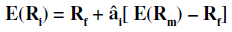
Where:
E (Ri) = Return required on financial asset i
Rf = Risk-free rate of return
âi = Beta value for financial asset i
E (Rm) = Average return on the capital market

---

Assumptions of CAPM

The CAPM is often criticized as being unrealistic because of the assumptions on which it is based, so it is important to be aware of these assumptions and the reasons why they are criticized. The assumptions are as follows:

• Investors hold diversified portfolios: This assumption means that investors will only require a return for the systematic risk of their portfolios since unsystematic risk has been eliminated and can be ignored.
  
  
• Single-period transaction horizon: A standardized holding period is assumed by the CAPM in order to make comparable the returns on different securities. A return over six months, for example, cannot be compared to a return over 12 months. A holding period of one year is usually used.
  
  
• Investors can borrow and lend at the risk-free rate of return: This is an assumption made by portfolio theory from which the CAPM was developed, and provides a minimum level of return required by investors.
  
  
• Perfect capital market: This assumption means that all securities are valued correctly and prices reflect all information.
  
  
• Homogeneous expectations: All investors analyze securities in the same way and share the same economic view of the world. The result is identical estimates of the probability distribution of future cash flows from investing in the available securities.
  
  
• Rational Investors: All investors are rational mean-variance optimizers. It means that at a given level of risk they want to maximize their return and for a given level of return they want to minimize their risk.

---

Inputs for CAPM

To apply the CAPM, you need to estimate the following factors:

• Risk-free rate of return
• Market risk premium
• Beta

Risk Free rate of Return

In theory, the risk-free rate is the minimum rate of return an investor expects for any investment with zero risk. In practice, however, the risk-free rate does not exist because even the safest investments carry a very small amount of risk.

However, short-term government debt is a relatively safe investment and in practice, return on these assets can be used as an acceptable proxy for the risk-free rate of return under CAPM. The risk-free rate of return is also not fixed, but will change with changing economic circumstances.

Market Risk Premium

Market risk premium is the difference between the expected return on a market portfolio and the risk-free rate. It results of investment in risky security rather than risk-free security. The market risk premium can be calculated as follows:

Market Risk Premium = Expected Return of the Market – Risk Free Rate

Beta

Beta is an indirect measure which compares the systematic risk associated with a company’s shares with the systematic risk of the capital market as a whole. If the beta value of a company’s shares is 1, the systematic risk associated with the shares is the same as the systematic risk of the capital market as a whole.

Beta can also be described as ‘an index of responsiveness of the returns on a company’s shares compared to the returns on the market as a whole’.

For example, if a share has a beta value of 1, the return on the share will increase by 10% if the return on the capital market as a whole increase by 10%. If a share has a beta value of 0.5, the return on the share will increase by 5% if the return on the capital market increases by 10%, and so on. Beta values are found by using regression analysis to compare the returns on a share with the returns on the capital market.

Beta can be calculated as fallow:

Beta = Cov (Ri,Rm)/Variance of Rm

Where:
Cov (Ri,Rm) = Covariance between individual security and market return
Ri= Individual security return
Rm= Market return

---

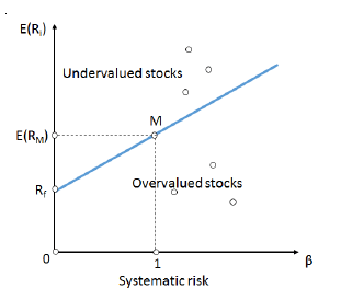
Security Market Line (SML)

The security market line (SML) is the line that reflects an investment’s risk versus its return, or the return on a given investment in relation to risk. The measure of risk used for the security market line is beta.

The SML essentially graphs the results from the capital asset pricing model (CAPM) formula. The x-axis represents the risk (beta), and the y-axis represents the expected return.

The market risk premium is determined from the slope of the SML. The relationship between â and required return is plotted on the securities market line (SML) which shows expected return as a function of â.

The intercept is the nominal risk-free rate available for the market, while the slope is the market premium, E (Rm) ?Rf. The securities market line can be regarded as representing a singlefactor model of the asset price, where beta is exposure to changes in value of the Market. The equation of the SML is thus:

Where:
E (Ri) = Return required on financial asset i
Rf = Risk-free rate of return
âi = Beta value for financial asset i
E(Rm) = Average return on the capital market

---

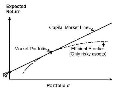
Capital Market Line (CML)

As discussed in the previous section, adjusting for the risk of an asset using the riskfree rate, an investor can easily alter his risk profile. Keeping that in mind, in the context of the capital market line (CML), the market portfolio consists of the combination of all risky assets and the risk-free asset, using market value of the assets to determine the weights.

The CML defined by every combination of the risk-free asset and the market portfolio. The Mean-Variance criteria as proposed by Henry Markowitz’ did not take into account the risk-free asset.

The CML results from the combination of the market portfolio and the riskfree asset. All points along the CML have superior risk-return profiles to any portfolio on the efficient frontier, with the exception of the Market Portfolio, the point on the efficient frontier to which the CML is the tangent.

From a CML perspective, this portfolio is composed entirely of the risky asset, the market, and has no holding of the risk free asset, i.e., money is neither invested in, nor borrowed from the money market account.

Where:
E(Ri)= Expected rate of return of portfolio (i)
Rf = Risk free rate of return
λ= slope of CML
σ = standard deviation of portfolio (i)

The slope of CML can be obtained as follow:

λ=E(Rm) – Rf/ σ

λ= Slope of capital market line
σ = standard deviation of market returns

Importance of Capital Assets Pricing Model (CAPM)

The CAPM is the most widely used risk return model. Its popularity may be attributed to the following factors:

• Some objective estimate of risk premium is better than a completely subjective estimate or no estimate.
  
  
• CAPM is a simple and intuitively appealing risk-return model. Its basic message that “diversifiable risk does not matter is accepted” by nearly every one.
  
  
• While there are plausible alternative risk measures, no consensus has emerged on what course to plot if beta is abandoned. As Richard Brealey and Stewart Myers say: “So the capital asset pricing model survives not from a lack of competition but from a surfeit”.

The situation perhaps may change as additional evidence is gathered in favour of arbitrage pricing model and operational guidelines for applying that model are developed further. As of now, however, the CAPM appears to be the model of choice in practice.

Implications of CAPM

• The CAPM has asset pricing implications because it tells what required rate of return should be used to find the present value of an asset with any particular level of systematic risk (beta). In equilibrium, every asset’s expected return and systematic risk coefficient should plot as one point on the CAPM.
  
  
  If the asset’s expected rate of return is different from its required rate of return, that asset is either under priced or overpriced. This implication is useful only if the beta coefficients are stable over time. However, in reality, the betas of assets do change with the passage of time as the assets’ earning power changes. The job of security analyst is, thus, to find the assets with dis- equilibrium prices, because it will be profitable to buy under priced assets and sell short the overpriced assets.
  
  
• With the help of CAPM, every investor can analyse the securities and determine the composition of his portfolio. Since, there is a complete agreement among investors on the estimates of expected return, variances and covariances and risk free rate, efficient set of portfolio should be the same for all the investors. Since all the investors face the same efficient set, the only reason they choose different portfolios is that they have different indifference curves.
  
  
  An indifference curve is the locus of all possible portfolios that provide the investor with the same level of expected utility. Expected utility will increase as one moves from lower indifference curve to a higher indifference curve. But on the same indifference curve, any point on the curve gives the same utility.
  
  
  Such curves are positively sloped and convex for risk averters, concave for risk seekers and horizontal for risk neutral investors. Thus, different investors will choose different portfolios from the same efficient set because they have different preference towards risk and return. It implies that each investor will spread his funds among risky securities in the same relative proportion adding risk free borrowing or lending in order to achieve a personally preference overall combination of risk and return. This feature of CAPM is often referred to as separation theorem.
  
  
• Another important implication is that no security can in equilibrium have a tangency to touch, either axis on risk return space. If an investor has zero proportion in such securities, the prices of these would eventually fall, thereby causing the expected returns of these securities to rise until the resulting tangency portfolio has a non-zero proportion associated with it. Ultimately everything will be balanced out.

When all the price adjustments stop, the market will be brought into equilibrium, subject to the following conditions:

• Each investor will like to hold a certain positive amount of each risky security.
  
  
• The current market price of each security will be fixed at a level where the number of shares demanded equals the number of shares outstanding.
  
  
• The risk free rate will be fixed at a level where the total amount of borrowings will be equal to the total amount of money lent.

As a result, in equilibrium the proportion of the tangency portfolio will correspond to the proportion of the market portfolio. The market portfolio is a portfolio consisting of all the securities where the proportion invested in each security corresponds to its relative market value. Where the

Relative market Aggregate value of the security = Value of a security / Sum of aggregate market values of all the securities

The market portfolio plays a very important role in the CAPM because efficient set consists of an investment in the market portfolio coupled with a desired amount of either risk free borrowing or lending. Tangency portfolio is commonly referred to as the market portfolio.

• For any individual investor, security prices and returns are fixed, whereas the quantities held can be altered. For the market as a whole, however, these quantities are fixed (at least in the short run) and prices are variable. As in any competitive market, equilibrium requires the adjustment of each security’s price till there is consistency between the quantity desired and quantity available. Therefore, is but reasonable and logical that historical returns on securities should be examined to determine whether or not securities have been priced in equilibrium as suggested by the CAPM.

---

Limitations of CAPM

Though the CAPM has been regarded as a useful tool for both analysts of financial securities and financial managers, it is not without critics. The CAPM has serious limitations in the real world, discussed as follows:

• One of the main limitations of CAPM is that it is impossible to test the model’s validity due to problems in defining market portfolio.
  
  
• Another limitation is that the theoretical grounds on which it is based cannot stand up to empirical scrutiny.
  
  
• It is also suggested that b is not the only risk that mattered.
  
  
• The CAPM is based on expectations about the future. Expectations cannot be observed but we do have access to actual returns. Hence empirical tests and data for practical use tend to be based almost exclusively on historical returns.
  
  
• Beta (systematic risk) coefficient is unstable, varying from period to period depending up on the method of compilation. They may not be reflective of true risk involved. Due to the unstable nature of beta it may not reflect the future volatility of returns although it is based on the post history. Historical evidence of the tests of Beta showed that they are unstable and they are not good estimates of future risk.
  
  
• CAPM focuses attention only on systematic (market related) risk. However, total risk has been found to be more relevant and both types of risk appear to be positively related to returns.
  
  
• Investors do not seem to follow the postulation of CAPM and do not diversify in a planned manner.
  
  
• The analysis of SML is not applicable to the bond analysis, although bonds are a part of the portfolio of the investors. The factors influencing bonds in respect of risk and return are different andnbe risk of bonds is rated and known to investors.

Thus, it can said that the applicability of CAPM is broken by the less practical nature of this model as well as complexity and difficulty of dealing with beta values.