
Portfolio Risk and Return Analysis
The expected return of a portfolio is computed by taking the weighted average of the expected return of the stocks in the portfolio. As the weighted average of the likely profits of the assets in the portfolio, weighted by the likely profits of each asset class, i.e., by using the following formula:

Here, Pi = The part of the portfolio invested in stock i
Ri = The expected return on stock i
The same formula can be simplified and written as:
E(R) = w1 R1 + w2 R2 + …+ wnRn
Table of Content
Consider the case of a portfolio in which we have two assets, namely mutual fund investing in bonds and mutual fund investing in stocks. The expected return on the bond-based mutual fund is 8% and the expected return from the stock-based mutual fund is 10%. The investment is divided between the two assets in the proportion of 70%-30%. Therefore, for this situation, the expected return would be:
E(P) = w1 R1 + w2 R2
E(P) = (0.7 * 0.08) + (0.3 * 0.10)
E(P) = 0.056 + 0.03
E(P) = 0.086 = 8.6%
Consider the case of a simple portfolio, which contains two mutual funds, wherein one of them is invested in bonds and the other one in stocks. Here, we expect the 6% return from the stock fund and 10% return from the bond fund and to each class, we have allocated 50%. In this scenario, we have the following values:
Expected return (portfolio) = (0.1)(0.5) + (0.06)(0.5) = 0.08 or 8%
Expected return is, by no means, an assured rate of return. Yet, it can be used to predict the future value of a portfolio. In addition, it provides a guide from which actual returns are measured.
Now consider another example. Let’s suppose an investment manager has created a portfolio with Stock A and Stock B. Stock A has an expected return of 30% and a weight of 40% in the portfolio. Stock B has an expected return of 15% and a weight of 60%. Then, the expected return of the portfolio can be calculated be as follows
E(R) = (0.40)(0.30) + (0.60)(0.15) = 12% + 9% = 21% The expected return of the portfolio is 21%. Now, let’s frame our knowledge of expected returns using the concept of variance.
Portfolio Variance
The variance of a portfolio is the measure of the volatility or the risk associated with it. Portfolio variance takes into account the standard deviation of each asset of the portfolio as well as the covariance of each asset of the portfolio with the others. The lower the covariance among the assets of the portfolio, the lower would be the portfolio variance.
Here, it is important to reiterate the key features of covariance, which are as follows:
- A positive covariance indicates that the return on assets moves together.
- A negative covariance means returns move contrary.
- Zero covariance indicates that there is no correlation between the two assets.
Mathematically, covariance is expressed as:
n
Cov (A, B) = {∑ (RA – (R’A)) i * (RB – (R’B)) i} / (n -1)
i = 1
Where,
Cov (A, B) = Covariance of asset A and asset B
RA = Return on asset A for period i
RB = Return on asset B for period i
R’A = Average of all the returns of asset A over the entire period
R’B = Average of all the returns of asset B over the entire period
n = Number. of periods
Let us understand covariance with the help of an example. Assume that there are two stocks S1 and S2. The closing price data for five days of the stock is shown in Table:
| Day | S1 Return (%) | S2 Return (%) |
|---|---|---|
| 1 | 1.2 | 3.3 |
| 2 | 1.8 | 4.1 |
| 3 | 2.2 | 4.8 |
| 4 | 1.3 | 4.0 |
| 5 | 0.25 | 2.56 |
Now, let us calculate the average return for each stock:
For S1, average return = (1.2 + 1.8 + 2.2 + 1.3 + 0.25) / 5 = 1.35
For S2, average return = (3.3 + 4.1 + 4.8 + 4.0 + 2.56) / 5 = 3.752
The Covariance for the above example is calculated as:
= [(1.2 – 1.35) x (3.3 – 3.752)] + [(1.8 – 1.35) x (4.1 -3.752)] + [(2.2 – 1.35) x (4.8 – 3.752)] + [(1.3 – 1.35) x (4.0 – 3.752)] + [(0.25 – 1.35) x (2.56 – 3.752)] / (5-1)
= [(-0.15 × -0.452) + (0.45 × 0.348) + (0.85 × 1.048) + (-0.05 × 0.248) + (-1.1 × -1.192)]/4
= [0.0678] + [0.1566] + [0.8908] + [- 0.0124] + [1.3112] / 4
= 2.414 / 4
= 2.414 / 4
Portfolio variance can be reduced by selecting assets that have low or negative covariance, such as bonds and stocks. Portfolio variance depends on the covariance or correlation coefficient of the securities in the portfolio. Portfolio variance is computed by multiplying the squared weight of each security by its corresponding variance and adding two times the weighted average weight multiplied by the covariance of all individual security pairs.
Thus, we get the following formula to calculate portfolio variance in a simple two-asset portfolio:
σ2 = w12 σ1 2 + w2 2 σ2 2 + 2 w1 w2 Cov(1,2)
Where,
w1 = Weight of Asset 1 in the portfolio
w2 = Weight of Asset 2 in the portfolio
σ1 2 = Variance of Asset 1 in the portfolio
σ2 2 = Variance of Asset 1 in the portfolio
Cov(1,2) = Covariance of asset 1 and asset 2
Let an investor have two assets, A and B, in the proportion of 60% and 40%. The return on A is 10% and that on B is 15%. From here, we can calculate the expected return, as follows:
E (P) = (.6.1) + (.4.15)
= 0.12 = 12%
The returns of the past five periods is shown in Table:
| N | RA | RB |
|---|---|---|
| 1 | 10% | 14% |
| 2 | 12% | 20% |
| 3 | 5% | 2% |
| 4 | 11% | 8% |
| 5 | 9% | 16% |
Table shows the calculation of the covariance of asset A with respect to asset B:
R’A = (10 + 12 + 5 + 11 + 9) / 5 = 9.4
R’B = (14 + 20 + 2 + 8 + 16) / 5 = 12
| N | RA | RB | RA– R’ A (R’ A = 9.4) | RB– R’ B (R’ B = 12) | (RA–R’a) (Rb–R’ B) |
|---|---|---|---|---|---|
| 1 | 10% | 14% | 0.6 | 2 | 1.2 |
| 2 | 12% | 20% | 2.6 | 8 | 20.8 |
| 3 | 5% | 2% | –4.4 | –10 | 44 |
| 4 | 11% | 8% | 1.6 | –4 | –6.4 |
| 5 | 9% | 16% | –0.4 | 4 | –1.6 |
| Sum | 58.00 |
We have to find the covariance of asset a with respect to the asset b.
The covariance will be: 58/4 = 14.5
Standard Deviation
Standard deviation can be defined as follows:
- A measure of the dispersion of a set of data from its mean. It indicates about the level of volatility of the asset.
- The square root of variance. The higher the dispersion, the higher is the standard deviation.
Example: Standard Deviation
Standard deviation (σ) is calculated by taking the square root of variance. Assume that the variance of an asset is 144. In that case, the standard deviation of that asset will be:
(144)1/2 = 12.00%
Let us now elaborate another example that takes into account the concepts of variance and standard deviation.
Example: Variance and Standard Deviation of an Investment.
Assume that we have a stock of PNG bank and the data shown in Table has been provided to us|:
| Case | Probability | Return | Expected Return |
|---|---|---|---|
| Worst Case | 10% | 10% | 0.01 |
| Base Case | 70% | 15% | 0.105 |
| Best Case | 20% | 18% | 0.036 |
Expected return is 15.1%.
Answer:
σ2 = (0.10)(0.10 – 0.151)2 + (0.70)(0.15 – 0.151)2+ (0.20)(0.18 – 0.151)2
σ2 = (0.10)(0.051)2 + (0.70)(0.001)2 + (0.20)(0.029)2
σ2 = (0.10)(0.002601) + (0.70)(0.000001) + (0.20)(0.000841)
σ2 = 0.0002601+ 0.0000007 +0.0001682
σ2 = 0.000429
The variance for PNG bank stock is .000429. Given that the standard deviation of a stock is simply the square root of the variance, the standard deviation is 0.0207.
Measuring Risk
There is a subtle difference between risk and return. The expected return of a portfolio is the weighted average of the individual returns. However, in case of risk the expected risk of portfolio is not the weighted average of the individual assets in the portfolio. The overall risk of the portfolio depends on the type of assets that comprise the portfolio. Generally, we can obtain a lower level of overall risk of the portfolio if we combine the assets ranging from risk-free or risk-less assets to the extremely risky assets in some fixed proportion.
We have already discussed two concepts related to portfolio risk, viz. variance and standard deviation. The variance is calculated by weighting each dispersion by its relative probability (take the difference between the actual return and the expected return, then square the number). The basic or the most frequently used measure of risk is the standard deviation. If there are two investment options under consideration then the option with lesser standard deviation will be preferred as it is assumed to be less risky
Investment Risk Measures
There are three indicators of investment risks apart from variance and standard deviation that are used to predict the volatility and return of a portfolio:
Beta: Also known as the beta coefficient, beta is the measure of a systematic risk. It is the measure of volatility of an individual security or the entire portfolio as a whole compared to the market as a whole. Beta is calculated using the regression analysis. The value of beta is an indicator of the stock movement with regards to the entire market. The value of beta may be 1, less than one or more than 1. The market is assumed to have a beta of 1.
The stock or any asset that has beta greater than 1 means that the stock has a greater expected risk and greater expected return that the market as a whole. For example, if the beta is 1.5, then the stock is 50% more volatile than the market as a whole. The stock or any asset that has beta less than 1 means that the stock has a lesser expected risk and lesser expected return that the market as a whole. For example, if the beta is 0.5, then the stock is 50% less volatile than the market as a whole.
Alpha: Is a complex measurement of stock price volatility based on the specific characteristics of the specific security. Alpha is a measure of performance of a stock or portfolio on a ‘risk-adjusted basis’. Alpha takes into account the volatility (i.e. price risk) of an asset and compares its risk-adjusted performance to an already established benchmark index. The return of the stock or portfolio in excess of the return on the benchmark index is termed as the alpha of the stock or portfolio.
Alpha = Portfolio Return – Benchmark Portfolio Return
Here, Benchmark Return (CAPM) = Risk-Free Rate of Return + Beta (Return of Market – Risk-Free Rate of Return)
Benchmark Return (CAPM) = Rf + β (Rm – Rf )
And
Alpha, α = Rp – [Rf + (Rm – Rf) β]
Where,
Rp = Portfolio Return – Benchmark Return
An alpha of 1.0 means the stock has outperformed the market by 1%. Similarly, an alpha of -1.0 means that the stock has underperformed as against market by 1%.
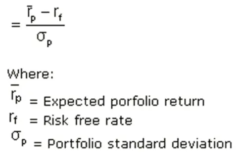
Sharpe Ratio: Is a complex measurement that utilises the standard deviation of a portfolio or stock to measure volatility. Greater is the Sharpe ratio, more is the potential return. Sharpe ratio is an indicator of stock performance taking into account the risk associated with it. It measures the excess return or the risk premium, per unit of deviation in the stock or portfolio. It is calculated using the formula mentioned below:
Sharpe Ratio = (total return – risk free rate of return) / standard deviation of portfolio
For example, let there be two managers M1 and M2. Assume that M1 earns 20% return and M2 earns 17% return. On the surface, it appears that M1 had performed better. There may be a case that M1 performed better because he took more risks than M2 and M2 has better risk-adjusted returns.
Assume that the risk free-rate is 5%, the standard deviation of M1 is 9% and the standard deviation of M2 is 6% Then, M1’s Sharpe ratio = 1.66 and M2’s Sharpe ratio = 2. Therefore, we see that M2 earned higher risk-adjusted returns.
Correlation Coefficient
Correlation coefficient is the measure of the degree of two variables with respect to each other. It is calculated as follows:
ρab = Cov (a,b) / (σa σb)
Where,
ρab = Correlation coefficient
Cov (a,b) = Covariance of asset a and asset b
σa σb = Standard Deviation of asset a and asset b respectively
Let us understand the coefficient of correlation by solving an example:
Cov(a,b) = 1.90
σa,= 0.8
σb = 2.2
ρab = 1.9 / (0.8 * 2.2)
ρab =1.079
Its value varies from -1 to +1, wherein -1 indicates perfect negative correlation and +1 indicates perfect positive correlation.
Risk premium can be defined as the return in excess of the risk-free rate of return that an investment yields. An asset’s risk premium is a kind of compensation for investors who bear the extra risk – compared to that of a risk-free asset in a given investment. Its formula is given below:
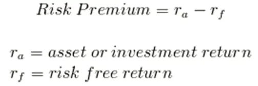
For example, assume that the expected return on a security is 19.5% and the risk free rate of return is 9.5% then the risk premium will be, 19.5% – 9.5% = 10 %.
If an investor has an option of investing in either blue chip funds or the funds of lesser known companies (startups which are not well established) in the market, then depending on his risk taking capacity he may invest in blue chip funds which are high yielding funds with very low risk of default or he may choose new funds in expectation of higher profits but these have uncertain profitability and higher risk of default.


