
Evaluation of Portfolio Performance
The rate of return of a portfolio is measured as the sum of cash received (dividend) and the change in the portfolio’s market value (capital gain or loss) divided by the market value of the portfolio when it was purchased. Mathematically, it can be expressed as follows:

Table of Content
Effective performance of portfolios depends a great deal on extensive research on market conditions. Portfolio managers sometimes attempt to invest on securities based on their intuition. This is the reason why some portfolios consistently fail. On the contrary, those who have a clear methodology and a rational attitude towards investing in different securities generally achieve high portfolio performance. The first step in portfolio research is to identify the determinants of portfolio performance.
Determinants of Portfolio Performance
There are three main determinants of portfolio performance, which are listed in Figure:
Asset Allocation
It is the major determinant of the long-term performance of a portfolio’s long-term return. Asset allocation is all about classifying an investment portfolio into three asset categories: stocks, bonds, and cash. The asset allocation that is the most appropriate for an organisation at a particular point in time depends on the time horizon and its ability for risk tolerance.
Risk and Returns
Risks and returns are the two inseparable part of any portfolio investment made by an organisation. Every investment of an organisation is subject to a certain degree of risk. Higher the risks associated with an investment, higher the chances are for good investment returns.
For instance, if an organisation has a long-term financial goal, it can target at achieving returns by investing in asset categories with greater risk, such as stocks or bonds. On the other hand, cash investments can be appropriate for financial goals having short time horizon as there are less risks involved in cash investments.
The rate of return is the most important measure of the outcome of a portfolio. The returns from a portfolio can be used to reinvest on securities or the investors may choose to withdraw the returns fund from their portfolios.
However, as much as it is important to calculate the returns of one’s portfolio, it is equally important to use the information to assess the risk associated with each security in the portfolio. J. L. Treynor introduced the component of risk in the measurement of portfolio performance. The objective of including risk in the measurement was to devise a performance measure that could be used by all investors, irrespective of their risk profiles.
Treynor suggested that there are two components of risk:
- Risks arising from market fluctuations
- Risks arising from the fluctuations of individual securities
Treynor gave the concept of security market line (SML) that gives the relationship between portfolio returns and market rates of returns. The slope of the security market line measures the relative volatility between the portfolio and the market. This is represented as beta coefficient, which measures the volatility of a stock portfolio to the market. The more the slope, the better is the risk-return trade off. This one-factor model, considering only beta (Capital Asset Pricing Model) implies that there is a linear relationship between an asset’s expected return and corresponding beta. However, beta alone cannot determine a portfolio’s returns.
Therefore, CAPM was expanded to include two other risk factors to better explain a portfolio performance:
Market Capitalisation
It is the value of an organisation’s shares outstanding multiplied by the current market price of the share. For example, if an organisation has 35000 shares outstanding, each with a market value of ₹100, the market capitalisation would be ₹35,00,000 (35,000 x ₹100 per share). Based on this, companies are grouped into large-cap, medium-cap, and small-cap organisations
Book Value/Market Value
Book value is the total value of an organisation’s assets that shareholders would receive if the organisation is liquidated. Market value is the current price of a share of a listed public limited organisation. When compared with market value, book value indicates whether the organisation is over or under-priced.
Market Cycles
These refer to trends or patterns in a given market environment, allowing some securities or asset classes to outperform others. For example, assets that are outperforming the market today may not perform well after some time. Every asset category has a unique cycle. Revenue and net profits may exhibit similar growth patterns among many companies within the same sector or industry.
However, it is an organisation’s resilience and preparedness to endure such underperformance of assets. Thus, it should be noted that a portfolio may not identically track the market every single year.
Methods of Calculating Portfolio Returns
Effective asset allocation is not only sufficient for an organisation to achieve its financial goals. An organisation needs to measure the performance of its portfolio within the decided time horizon. As discussed earlier, the performance of portfolio is measured in two ways: one is to calculate returns on investment and the other is to estimate risk content of the investment. In this section, a focus is given on measuring portfolio performance by calculating associated returns. Organisations use different methods for calculating returns on investment.
These methods are explained in detail in the subsequent sections.
Money Weighted Rate of Return
An assessment of the profit rate for an asset or portfolio of assets is called money weighted rate of return. It can be estimated by calculating the rate of return that will fix the current values of all cash flows and terminal values same as the value of the first investment. The money weighted rate of return is same as the internal rate of return (IRR). This is because it ascertains that the similar rate of return is achieved during every sub-period of the possibility of an investment.
The money weighted rate of return includes the size and schedule of cash flows; thus, it is an effectual amount for portfolio returns. Money weighted rate of return is the discount rate at which the NPV=0. In other words, it is the rate at which the present value of inflows is equal to the present value of outflows. In the IRR calculation, all cash inflows and outflows are identified.
In terms of an investment portfolio, cash outflows and cash inflows would be as follows:
Cash outflows:
- The cost of any investment purchased
- Reinvested dividends or interest
- Withdrawals
Cash inflows:
- The proceeds from any investment sold
- Dividends or interest received
- Contributions
Each inflow or outflow needs to be discounted back to the present using a rate (r) which would make Present Value of inflows = Present Value of outflows. Let us look at an example.
Illustration: Kartik purchases one share of a stock for ₹50 that pays an annual ₹2 dividend, and sells it after two years for ₹65. In this case, the money-weighted rate of return would be the rate satisfying the following equation:

Using a spreadsheet or financial calculator and solving for r, the money-weighted rate of return = 17.78%.
It is important to note that the main drawback of the money-weighted rate of return is that is cannot serve as a tool for evaluating managers. In addition, Money-weighted rate of return takes into account all cash flows, including contributions and withdrawals. Supposing a money-weighted return is calculated over ceratin time periods, the formula tends to give greater weightage to the periods where portfolio size is the largest.
Linked Internal Rate of Return
The Linked Internal Rate of Return (LIRR) is used to estimate the accurate time weighted rate of return (TWRR). In this method, the internal rate of return is calculated over consistent time periods, and the outcome is associated geometrically. The following formula can be used to calculate LIRR:
LIRR= (1+R1 ) × (1+R2 ) × (1+R3 ) ×….. (1+Rn) – 1
Where R is the internal rate of return at different time periods.
Illustration: A mutual fund achieved quarterly MWRR of 4%, 9%, 5% and 11% during 2013. Calculate the LIRR.
LIRR = (1+0.04) × (1 + 0.09) × (1 + 0.05) × (1 + 0.11)- 1
LIRR = (1.04) × (1.09) × (1.05) × (1.11) -1
Therefore, LIRR = 1.32 – 1 = 0.32 or 32%
If the consistent time intervals are not years, the un-annualised investment time adaptation of IRR for each period or the IRR for every time period should be estimated. After that, each IRR should be converted into the investment period return over the time period and investment period profits should be connected to get the LIRR.
Modified Dietz Return
Modified Dietz return is a simple interest estimate of Money Weighted Returns. The formula is named after Peter Dietz who developed the return calculation method. The Modified Dietz method provides a computational advantage over the IRR method as it is a closed form solution and does not require several trial and error exercises before arriving at the final figure. The calculation takes into account the cash flows that have been adjusted to reflect the time they were available for investment in the portfolio.
The formula to calculate Modified Dietz return is as follows:
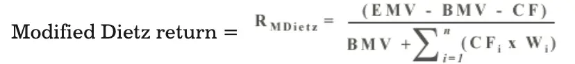
Where,
EMV = It is the market value of the portfolio at the end of the period, including all income accrued up to the end of the period.
BMV = It is the portfolio’s market value at the beginning of the period, including all income accrued up to the end of the previous period.
CF = This is the net cash flows within the period where contributions to the portfolio are positive flows or inflows and withdrawals or distributions are referred to as negative flows or outflows.

Wi , Wi is the proportion of the total number of days in the period that cash flow CFi has been held in (or out) of the portfolio. The formula for Wi is as follows:

Where,
CD = Total number of calendar days in the period
Di = The number of calendar days since the beginning of the period in which cash flow CFi occurred. The numerator is based on the assumption that cash flows occurred at the end of the day. Suppose a cash flow occurred on January 20th (January has 31 days), the ratio Wi would be calculated as (31–20)/31 = 0.35. This is the cashflow adjustment factor.
Let us understand the calculation with the help of an example.
The portfolio investment from 31-March, 2014 to 30- April, 2014 is shown in the following table:
| Date | Number of Days Invested | Day Weight | Value |
|---|---|---|---|
| 31-March-2014 | 30 | 1.00 | 100 |
| 20-April- 2014 | 10 | 0.33 | 10 |
| 30-April-2014 | – | – | 120 |
Calculate the Modified Dietz return.
Solution: Beginning market value + Accrued Income (BMV) = 100
Ending market value + Accrued Income (EMV) = 120
Cash flow on 20th April = 10
Adjustment factor = (30-20)/30 = 10/30 = 0.33
Adjusted cash flow = 10 × 0.33 = 3.3

True Time Weighted Rate of Return
The true time weighted return method is used to measure portfolio return indifferent towards cash inflow and outflow of a portfolio. Unlike the Dietz or internal rate of return, the true time weighted return does not use money weighted estimations. In place of that, the true timeweighted return method estimates the return of the portfolio as time weighted average of its component’s return, in spite of cash add-ons and extractions to the portfolio. The true time weighted return is used by StatPro Revolution.
Let us understand the true time weighted return method with the help of an example. Suppose a portfolio’s value was ₹1000 at the start of the month and ₹1900 towards the end of the month. On the 10th day, ₹250 has been deposited, and another ₹250 has been deposited on the 20th day. The total value of the portfolio, after the deposits, is ₹1,300 on the 10th day, and on the 20th day the deposit is ₹1,700. Hence, 1 to 10, 11 to 20, and 21 to 30, are the three sub-periods.
To measure the time weighted return, the return of each sub period has to be measured.
- The return of the first sub period is :[(₹1,300-$250)-$1,000] / $1,000 = 5%.
- The return of the second sub period is: [ (₹1,700-$250)-$1,300 ] / $1,300 = 11.5%
- The return of the third sub period is: [ (₹1,900-$1,700) ] / $1,700 = 11.8%
Lastly, the total returns are estimated to calculate the total time weighted rate of return.
Time-weighted rate of return: [(1+0.05)(1+0.115)(1+0.118)]^0.33 -1 = 9.39%
Risk-Adjusted Performance Measures
Risk-adjusted performance measures are the metrics that analyse the return on investment with a few alterations for the threat. It could be income, gains, returns, and so on. In the same way, volatility, beta, value at risk is some of the ways in which the threat can be estimated. In finance, different risk-adjusted performance measures are engaged.
In the 1960s, some were created for examining the competency of the market theory, which are now used by practitioners for asset allotment and presentation evaluation. They are Treynor ration, Sharpe ratio and Jensen’s alpha. Return on Capital (ROC) and Risk-adjusted Return on Capital (RAROC) are other risk-adjusted performance measures created in the 1980s and 1990s to back financial capital allowance. Let us discuss some of the methods of risk-adjusted performance measures in the subsequent sections.
The Sharpe ratio, also called the Sharpe index or the Sharpe measure or the reward to variability ratio, in finance, ascertains the performance of an investment by regulating the risk. This method is named after William Forsyth Sharpe. The ratio estimates the excess return or risk premium for each unit of deviation in the investment asset or trading strategy, classically referred to as risk.
The Sharpe ratio also referred to as Sharpe index measures the performance of a portfolio in a given period of time. To compute the Sharpe ratio, one must know three things, the portfolio return, and the risk free rate of return and the standard deviation of the portfolio. The Sharpe index is computed by dividing the risk premium of the portfolio by its standard deviation or total risk.
Mathematically, the Sharpe index is given as follows:
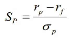
Where,
rp = Portfolio rate of return
rf = Risk free rate of return
σp = Standard deviation
The Sharpe index uses the capital market line as a benchmark.
Let us understand this with the help of the following illustration:
Illustration: A portfolio manager attained a return of 15% on a portfolio. The standard deviation is 0.3 and the market realised a return of 14.6%. The risk-free rate of return is 7%. Calculate the Sharpe Index.
Solution:
rp = 0.15
rf = 0.07
σp = 0.3
Therefore Sharpe index Sp = 0.15 – 0.07 / 0.3 = 0.267
Treynor’s Reward to Volatility
The Treynor ratio, also known as the reward to volatility ratio or Treynor measure and named after Jack L. Treynor, is a method used to estimate how well a portfolio has compensated its investors at the given risk level. This method relies on beta, which is the sensitivity of an investment to market fluctuations, in order measure associated risk content.
The Treynor ratio is the most appropriate method for comparing two investments of the same category or to an investment’s Treynor ratio with that of a market benchmark. Investments having a low beta are less volatile, thus have less risks and lower potential return. On the other hand, investments with a high beta indicate higher risks and higher potential returns.
To measure risks associated with an investment using the Treynor ratio, the following three inputs are required:
- The arithmetic average return over a specific time frame of the investment
- The arithmetic average return for a risk-free investment over that same time frame
- The investment’s beta during that period
To estimate the investment’s excess returns, the average return on the riskless asset is subtracted from the average return of the portfolio. The result is further divided by the investment beta (estimated by comparing the investment’s excess returns during a given time period with those of the benchmark) to calculate the Treynor ratio.
The Treynor’s ratio is useful for assessing the excess return, helps investors to evaluate how the portfolio structure to different levels of systematic risk that would affect the return. Mathematically, the Treynor Index (Tp) is given as follows:
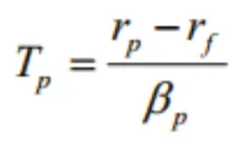
Where,
rp = Portfolio rate of return
rf = Risk free rate of return
βp = Portfolio beta
When rp > rf and βp > 0, a higher Treynor’s index is achieved, which implies a better portfolio investors regardless of risk profiles.
Two cases in which the Treynor ratio may be negative are as follows:
- When rp < rf: Treynor index is negative and the portfolio performance is evaluated as being very poor.
- When βp < 0: The negativity is owing to beta, which means risks are low and fund performance is excellent.
Let us understand this with the help of the following illustration:
Illustration: The following data is related to three funds namely, ABC, DEF and GHI, with their rate of return and beta. The risk-free rate is 12%. The risk for market (M) is 1.0 and the rate of return for the market (M) is 18%.
| Manager | Rate of Return | Beta |
|---|---|---|
| Market | 18% | 1 |
| ABC | 16% | 0.90 |
| DEF | 20% | 1.05 |
| GHI | 22% | 1.20 |
Using Treynor’s ratio, calculate the value of each manager.
Solution:
- For market: rp= 18%, rf = 12%, βM = 1.0
Substituting the values in the formula: Tmarket = (0.18 – 0.12)/1 = 0.06 - For manager of ABC: rp= 16%, rf = 12%, βM = 0.90
TABC = (0.16 – 0.12)/0.90 = 0.044 - For manager of DEF: rp= 20%, rf = 12%, βM = 1.05
TDEF = (0.20 – 0.12)/1.05 = 0.076 - rp= 22%, rf = 12%, βM = 1.20
TGHI = (0.22 – 0.12)/1.20 = 0.083
Compared to the market, the Treynor’s ratio for DEF and GHI are higher. ABC could not beat the market’s performance. Of the three funds, the manager of fund GHI outperformed the rest.
Jensen’s Alpha
Jensen’s alpha or Jensen’s Performance Index, ex-post alpha, in finance, is used to ascertain the irregular return of a security or portfolio of securities over the hypothetical anticipated return. The method is based on the perception that assets that are more vulnerable have more anticipated returns as compared to less vulnerable ones. Jensen index utilises the security market line as a benchmark. The measure was first used for evaluating the mutual fund managers.
The Jensen’s model is used to adjust the level of beta risk, so that riskier securities are expected to have higher returns. The index allows the investor to statistically evaluate whether a portfolio produced an abnormal return relative to the overall capital market. An important point to consider while using the Jensen’s index is the choice of the market index as the portfolio performance is compared to the market portfolio.
According to capital asset pricing model (CAPM), in an equilibrium risk return model, the expected rate of return on an asset or portfolio is expressed as follows:
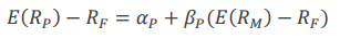
Where,
Erp = Expected return of an asset or portfolio
rf = Risk free rate of return
Erm = Expected return on the market portfolio
βp = Beta or systematic risk of the asset or portfolio
For obtaining Jensen’s ratio, time series regression of the security’s return (rp – rf )is regressed against the market portfolio excess return (rm – rf ) .
Therefore,
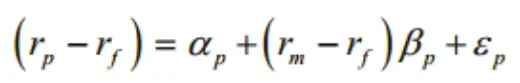
Where, rp = return on the portfolio
rf = Risk free rate of return
αp = Jensen Index measure of the performance of the portfolio
βp = Beta or systematic risk of the portfolio
rm = Return of the market portfolio
εp = Portfolio random error term
By taking the mean on the both sides,

The average error term εp is always zero.
Therefore, Jensen’s alpha (αp) can be written as follows:

To calculate Jensen’s alpha, one needs to first calculate the CAPM return.
CAPM return = Rf + β(Rmkt – Rf)
Where Rf = risk-free return and Rmkt = (average or “expected”) market return.
β= 1.470, Rmkt = 0.117%, Rf = 0.01%
Therefore, CAPM return = 0.01+ 1.470 (0.117 – 0.01) = 0.167%
Return of stock for the period = 0.66
Jensen’s alpha = Rstock – [ Rf + β (Rmkt – Rf )] where Rstock = (average or “expected”) stock return.
Jensen’s alpha = Rstock – CAPM
Therefore, Jensen’s alpha = 0.66 – 0.167 = 0.493%
Relative Risk of Mutual Funds
Mutual funds are basically a collection of stocks, bonds, and other financial assets. These funds are owned by a number of investors and managed by an investment management organisation. An investor in a mutual fund owns a share of the fund that is equal to the amount of his/her investment divided by the total value of the fund. Mutual funds are beneficial to investors especially to those who are just beginning to invest. Mutual funds selected after a thoughtful consideration and thorough market research can help investors in achieving their financial goals.
The following are the benefits of mutual funds:
- As a mutual fund is a collection of a number of securities, the performance of the fund does not depend on any single security; thus, the risk is shared among various securities.
- Investors need to pay high transaction costs while purchasing individual securities. Mutual funds provide the benefit of economies of scale to investors as it is a combination of different securities. Here, the economies of scale imply that mutual fund costs decrease with an increase in the asset’s size.
- Money invested in mutual funds is generally liquid; thus investors can redeem these funds on demand and collect their money.
- One of the methods to measure the performance of mutual funds involves comparison of the yields of different mutual funds, including an unmanaged portfolio. The popular holding period return formula is expressed as follows:
Holding Period Return =Income + (End of Period Value – Initial Value) / Initial Value
For example, suppose an investor purchased a stock a year ago at ₹5000and received ₹500 in dividends over the year. What would be the HPR for the investor, if the stock is now trading at ₹6000? HPR = [500 + (6000– 5000)] / 5000 = 0.3 = 30%
The performance of each mutual fund is compared with one another to decide on the outperforming fund. However, a portfolio manager should also consider the relative risk of portfolios. This is because a high performing mutual fund may be accompanied with higher risks as well. A mutual fund performance is also calculated using the Sharpe’s ratio, beta and Jensen’s alpha to include the associated risks
Table shows the risks associated with mutual funds:
| Type of risk | Type of investment affected | How the fund could lose money |
|---|---|---|
| 1. Market risk | All types | The value of investments goes down due to obligatory risks that influence the whole market |
| 2. Liquidity risk | All types | An investment cannot be sold whose value is decreasing since there is no one to buy them. |
| 3. Credit risk | Fixed income securities | If a bond giver is not able to repay a bond, it can result in insignificant investment. |
| 4. Interest rate risk | Fixed income securities | The value of fixed income securities decreases when the interest rates go up. |
| 5. Country risk | Foreign investments | The value of an unrelated investment goes down due to political changes or unsteadiness in the country where the investment was given. |
| 6. Currency risk | Investments denominated in a currency other than the Canadian dollar | If any other currency decreases against the Canadian dollar, the value of the investment goes down. |
Let us understand the performance evaluation of mutual funds with the help of an illustration:
Illustration: The following data relates to four mutual funds P,Q,R, and S. Rank the mutual funds using (a) Sharpe’s ratio, and (b) Treynor’s measure. The risk free rate of return is 8%.
| Mutual Fund | Average Annual Return | Standard Deviation | Correlation with Market |
|---|---|---|---|
| P | 22 | 15 | 0.75 |
| Q | 15 | 10 | 0.50 |
| R | 19 | 22 | 0.35 |
| S | 12 | 7 | 0.90 |
| Market portfolio | 12 | 10 |
Solution:
- Fund P = (0.22 – 0.08)/0.15 = 0.93
- Fund Q = (0.15 – 0.08)/0.10 = 0.70
- Fund R = (0.19 – 0.08)/0.22 = 0.50
- Fund S = (0.12 – 0.08)/0.07 = 0.57
Treynor’s ratio for the mutual funds is calculated as follows:
βp = Covariance of Market Return with Stock Return / Variance of Market Return
Also, beta coefficient equals correlation coefficient multiplied by standard deviation of stock returns divided
β = ( Correlation Coefficient between Market and Stock ) × (Standard Deviation of Stock / Standard Deviation of market return )
The beta for funds P, Q, R, S:
- Fund P = (0.75)(0.15)/0.10 = 1.125
- Fund Q = (0.50)(0.10)/0.10 = 0.50
- Fund R = (0.35)(0.22)/0.10 = 0.77
- Fund S = (0.9)(0.07)/0.10 = 0.63
Therefore, Treynor’s ratio for each of these funds would be:
- Fund P = (0.22 – 0.08)/1.125 = 0.124
- Fund Q = (0.15 – 0.08)/0.50 = 0.140
- Fund R = (0.19 – 0.08)/0.77 = 0.143
- Fund S = (0.12 – 0.08)/0.63 = 0.063
Fund ranking:
| Sharpe’s Ratio | Treynor’s Index |
|---|---|
| P | R |
| Q | Q |
| R | P |
| S | S |
Mutual Funds Vs. Benchmark Indexes
Mutual Funds
When an investment is made in the mutual fund, risks are shared by a group of investors. Thus, the most important aspect of funds is that they are less unpredictable. Individual stocks at times can be nullified, but if the mutual fund holds 50 stocks, it is improbable that all 50 of these stocks would become valueless. The other side of this lessened instability is that fund returns can be subdued compared to individual stocks. In investing, risk and return are related to each other.
Benchmark Index
Market benchmarks are used by investors, portfolio managers, and researchers for determining how a particular market performs. Market indexes are especially helpful for mutual fund investors as they offer market standards that help in the evaluation of risk and return history of their investments. Benchmark index is basically a tool that enables an investor to evaluate the performance of a fund by providing a point of reference.
In India, BSE Sensex and Nifty are most widely used benchmarks for large-cap funds. Other benchmarks include CNX Midcap, CNX Smallcap, CNX IT, CNX 500, BSE 200, BSE 100, etc. Therefore, if an investors has put his money in a diversified equity fund, it could be benchmarked against the BSE Sensex, and the return could be compared with that of BSE Sensex for evaluating the performance.
The performance of a mutual fund vis-a-vis the market benchmark is measured as Beta. Beta measures the volatility of a mutual fund compared to its benchmark. If the beta of the mutual fund is 1.10, he investors can expect 10% higher returns than the benchmark in an upward market, and 10% lower returns than the benchmark in a downward market. A beta of 1 indicates that the mutual fund would fluctuate in sync with the benchmark.


