
Markowitz Model
A Nobel Memorial Prize winning economist, Harry Markowitz devised the modern portfolio theory in 1952. Markowitz’s hypothesis emphasised the relevance of portfolios, risk, the correlations between securities and diversification. His work altered the manner in which people invested.
Before Markowitz’s theories, investors focused on what was placed on picking single high-yield stocks without any consideration to their impacts on portfolios as a whole. Markowitz’s portfolio hypothesis would be a huge initiative for the formation of the capital asset pricing model.
Table of Content
Formulation of Model
Harry Markowitz defined this model in 1952. It helps in the choosing the most effective portfolio by observing different probable portfolios of the stated securities. By selecting securities that do not ‘move’ precisely in concert, the HM model demonstrates investors the method to lessen their risk. In other words, the underlying principle of the model is that the combined risk of two securities would be different from the individual risk of the securities.
For example, according to the HM model, we can combine one security of TESCO and one of Relianceand get a portfolio, the risk of which will be different from the individual securities of Reliance or TESCO. The HM model is also known as Mean-Variance model because it is dependent on the expected returns (mean) and the standard deviation (variance) of the different portfolios.
Harry Markowitz made the following hypothesis while building the HM model:
- Risk of a portfolio is dependent on the variability of returns from the known portfolio.
- An investor is risk reluctant.
- An investor chooses to augment consumption.
- The investor’s utility function is concave and enhancing, because of his risk repugnance and consumption choice.
- Study is dependent on the single period model of investment.
- An investor also maximises his portfolio return for a given level of risk or increases his return for the least risk.
- An investor is balanced in character. To decide the best portfolio from a number of potential portfolios, every diverse return and risk, two split decisions are to be performed:
- Purpose of a series of effective portfolios
- Choosing the finest portfolio out of the effective series
Following are the major advantages of the HM model:
- It provides an effective mean of mitigating risks with the help of diversification.
- It helps in quantifying the benefits of diversification of a portfolio.
However, one important disadvantage of the HM model is that it is a complex and involves tedious calculations.
Efficient Frontier Calculation Algorithm
In the previous section, we studied the meaning, shape and properties of efficient frontier. Now, we will discuss how the efficient frontier can be calculated with the help of an algorithm. The Markowitz model is based on the assumption that portfolios face no constraints whatsoever. However, in reality there are many constraints that portfolios face.
For example, when short-selling is prohibited, it would be assumed by default that all the assets are positively weighed. In order to decide a certain portfolio diversification, the amount invested per security needs to be limited.
Thus, it is necessary to integrate the different constraints into resolution methods:
Typically, constraints are represented as follows:
ai ≤ xi ≤ bi , i = 1, …..,n
The impossibility to short sells is due to a special case where:
ai = 0 and bi= 1, i = 1, …..,n
Markowitz proposed an algorithm, called the critical line algorithm. This algorithm allows for the composition of efficient frontier portfolios to be determined when the proportions of assets are subject to constraints. Later, Sharpe proposed a description of this algorithm in a publication in 1970. The investor’s objective function is given as a function of the investor’s aversion to risk, represented as λ. By varying λ values, the characterisation of the complete efficient frontier is obtained.
The efficient frontier thus derived is a linear system where for each value of λ, the proportions of the optimal portfolio are derived. If constraints exist on the portfolio, then for each value of λ, the solution would have xi values equal to their lower limit, xi values located between their lower limit and their upper limit and xi values having upper limits. Assuming that each variable is known, linear equations can be derived. The value of each variable depends on the value of λ.
For each variable, a critical value of λ exists, which can be calculated according to the parameters of the problem. Later, the critical λ thus obtained are sequenced together to give the resolution algorithm. The resolution algorithm helps in finding the solution that is valid up to the first critical λ. This is continued making necessary modifications each time a variable changes status. The portfolios that correspond to the critical λ are referred to as “corner” portfolios. These portfolios are sufficient for calculating the complete efficient frontier.
Let us assume that we need to compute the efficient frontier using n assets. In order to do the computations, we need to have two inputs:
- Expected average return of the assets. We can denote the vector of expected result as Z.
- The variance-covariance matrix for the n assets. We can designate the covariance matrix as S. We even require a unity vector (1) with the similar length as the vector, Z.
When we have the data, we can run the computations using a matrix dependent on arithmetical program like Octave, as follows:
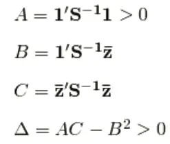
Using these values, the variance at each level of expected return is given by the equation:
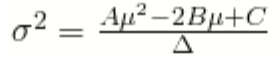
From the equation, you can see that the efficient frontier is a parabola in mean-variance space. Using standard deviation rather than variance, we have:
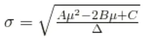
After calculating standard deviation, an investor can determine the expected return of a portfolio. For example, consider the following stock data collected by an investor:
| Expected Return | Standard Deviation | |
|---|---|---|
| Stock A | 20% | 30% |
| Stock B | 25% | 40% |
Let us assume there is a perfectly negative correlation between the returns of the two stocks. Now, we have to calculate the expected return of the portfolio in case the investor wants to get zero standard deviation in the return of the portfolio.
The weight of the stock A in the portfolio would be = 40/ (30+40) = 40/70 = 0.57
Therefore, the weight of stock B in the portfolio would be 1-0.57 = 0.43
The expected return of the portfolio would be = 0.5720% + 0.4325% = 11.4% + 10.75% = 22.15 %.
Other Algorithms
We have mentioned earlier that the Markowitz model involves tedious calculations. This is because we need to calculate and invert the correlation matrix. In addition, we have limited access to mechanical calculation at the time when the model was first introduced. Therefore, different experts have given different algorithms to reduce the complexity of the Markowitz model.
The Wolfe method (1959) was one of the first alternative algorithms to be proposed. The underlying principle of the Wolfe method is turning the initial quadratic problem to a linear problem, which can be calculated with the help of the simplex method. The Wolfe method results in a significant reduction in the calculation time of the Markowitz model. Many experts have also proposed using gradient methods to build portfolios using the Markowitz model.
Boots (1964) and Luenberger (1984) are some of the main proponents of these methods. William Sharpe worked on simplifying the Markowitz model and developed an empirical market model. The Sharpe model helps in reducing the number of calculations with the help of a relatively simple asset correlation structure. In addition, quadratic resolution methods were also introduced in the late 1990s to simplify stock selection. Elton and Gruber (1995) also introduced an optimisation model based on the Sharper`s market model.
Earlier we discussed that the Markowitz model is based on the premise that by diversification investors can mitigate risk or get a better return from a given level of risks. In this theory, Markowitz shows that the variance of the rate of return of a portfolio is a significant measure of the portfolio risk.
Therefore, the Markowitz model states that diversification can reduce risk. In addition, the model also provides a way of effectively diversifying risks. However, there are a number of limitations of this model which need to be resolved. One of the most commonly cited difficulty of the model is that it involves increasingly complex mathematical calculations as we increase the number of securities.
For example, for calculating the variance of the portfolio, we need to determine the covariance between each set of securities. The covariance of each pair of securities is shown in the covariance matrix. Naturally, when large number of securities is involved, we get a large covariance matrix which will involve highly complex calculations.
For example, in the case of n number of securities, we would require n number of variance terms and n (n-1) / 2 covariance terms. Because of this difficulty in calculation in this model, portfolio analysts avoid this model. In order to simplify the Markowitz model, William F. Sharpe developed the Single Index Model (SIM). This model helps in estimating the returns of securities as well as the value of the index.
The Sharpe`s SIM expressed the return from an individual security as a function of the return of the overall market index. This is shown in the following formula:
Ri = ai + bi RM + ei
Where,
Ri refers to the return on security i
RM refers to the return on the market index
ai refers to risk free return
bi is a measure of the sensitivity of the return of the security ‘I’with respect to the index return
ei refers to the error term
The single index model is a much simpler model than the Markowitz model. For example, if an investor is calculating for n securities, the single index model needs 3n+2 estimates; whereas the Markowitz model would require n (n+3) / 2 estimates. Therefore, in case of 50 securities, the Markowitz model would require 50*53/2 = 1325 estimates whereas the single index model would require only 152 estimates.


