What is Producer Equilibrium?
Producer equilibrium implies a situation in which a producer maximizes his/her profits. Thus, he /she chooses the quantity of inputs and output with the main aim of achieving the maximum profits.
Table of Content
In other words, he/she needs to decide the appropriate combination among different combinations of factors of production to get the maximum profit at the least cost. Least cost combination is that combination at which the output derived from a given level of inputs is maximum or at which the total cost of producing a given output is minimum.
Producer Equilibrium Example
Let us learn producer’s equilibrium with the help of an example. Suppose a producer wants to produce pencils with a total expenditure of ₹1500. The factors of production to produce pencils involve labour and capital, where the price of labour is 50/ unit and the price of capital is ₹75 per unit.
He can hire 30 units of labour with no capital or 20 units of capital with no labour. However, for producing pencils, he wants to have the optimum combination of both the factors. This can be explained with the help of Figure 1:
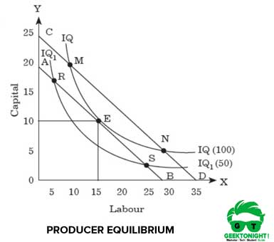
In Figure 1, the optimum combination is depicted by point E, where 10 units of capital and 15 units of labour are used. At point E, isoquant curve IQ is tangent to iso-cost line AB. The producer can produce 1500 units of output by using any combinations that are E, M and N, on curve IQ.
He/she would select the combination that would obtain the lowest cost. It can be seen from the Figure 1 that E lies on the lowest iso-cost line and would yield same profit as on M and N points, at the lowest cost. In such a case, E is the point of equilibrium; therefore, it would be selected by the producer.
Expansion Path
Expansion path can be defined as the locus of all the points that show least combination of the factors corresponding to different levels of
output. The expansion path is also called scale line as the expansion of the organization is based upon the scale of operation.
As per Stonier and Hague, “expansion path is that line which reflects the least cost method of producing different levels of output, when factor prices remain constant.”
Expansion Path Example
Let us learn the concept of the expansion path with the help of Figure 2:
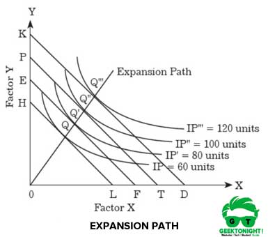
As shown in Figure 2, earlier the producer was producing 60 units of output. Suppose the producer wants to expand his/her production and wants to produce 80 units of output.
The equilibrium would be achieved at the point Q’, where the iso-cost line is tangent to an isoquant curve of IP’. Similarly, the equilibrium point for producing 100 and 120 units are Q’’ and Q’’’, respectively. When the points Q, Q’, Q’’ and Q’’’ are joined, a straight line is obtained, which is called the expansion path.
Business Economics Tutorial
(Click on Topic to Read)
Go On, Share article with Friends
Did we miss something in Business Economics Tutorial? Come on! Tell us what you think about our article on Producer Equilibrium | Business Economics in the comments section.
Business Economics Tutorial
(Click on Topic to Read)