Consumer Equilibrium: Effects on Income, Substitution, Price

What is Consumer Equilibrium?

Consumer Equilibrium refers to a situation where the consumer has achieved the maximum possible satisfaction from the quantity of the commodities purchased given his/her income and prices of the commodities in the market.

The ordinal utility approach (which follows the two-commodity model explanation) provides two conditions with respect to consumer equilibrium:

• First order condition
• Second order condition

The first order condition for consumer equilibrium in ordinal utility is
the same as that specified through cardinal utility. Therefore,

MU_x / MU_y = P_x / P_y

As MU_x / MU_y = MRS_x,y the first order condition in ordinal utility is given as follows:

MRS_x,y = MU_x / MU_y = P_x / P_y

The second order condition states that the first order condition must be satisfied at the highest IC as shown in Figure 1.

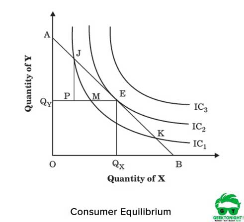
In Figure 1, IC1, IC2, and IC3 represent the hypothetical indifference map of a consumer. AB is the budget line that intersects IC2 at point E. This implies that the slope of IC2 and AB are equal. This satisfies both the first order condition and the second order condition.

In Figure 1, between any two points on an indifference curve, IC1:

∆Y. MU_y = ∆X. MU_x

Therefore, the slope of the curve would be:

∆Y / ∆X = MU_x / MU_y

The slope of budget line is given as:

OA / OB = P_x / P_y

At point E where MRS_y,x = P_x / P_y

Therefore, the consumer is at equilibrium at point E. As the IC2 curve is tangent to the budget line AB, IC2 is the highest indifference curve that a consumer can attain at the given income level and market price of commodities. At point E, the consumer consumes quantities OQx of X and OQy of Y to yield maximum satisfaction. In Figure 1, when the consumer is at point J and moves to point M, there is no difference in the satisfaction level at both points that lie on the same curve IC1.

However, as point E is the point of equilibrium, a consumer would tend to reach point E from J or M. The other point to note here is that the indifference curve IC3 is impossible to reach for the consumer due to budgetary constraints. His/her income does not permit the consumer to purchase any combination of commodities X and Y on indifference curve IC3.

The above explanation of the consumer equilibrium is based on an assumption that the income of the consumer and the market price of commodities remain unchanged.

However, this is not always the case as both income and market price may vary at different time periods. The change in these variables results in an upward or downward shift in the consumer’s budget line. The effects of these changes are shown in Figure below:

Also Read: Law of Diminishing Marginal Utility

Income Effect on Consumer Equilibrium

Income effect on consumer’s equilibrium can be defined as the effect caused by changes in consumer’s income on his/her purchases while the prices of commodities remain unchanged. Figure 2 illustrates the effect of change in the consumer’s income on his/her equilibrium:

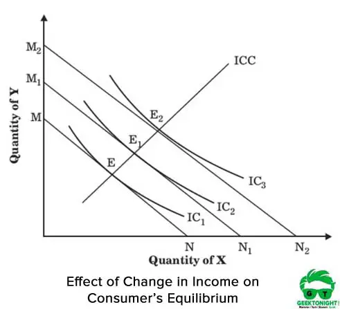
Point E is the original point of consumer’s equilibrium. At point E, the indifference curve IC1 is tangent to the budget line MN. In case the consumer’s income increases, the budget line would shift from MN to M1N1 and then to M2N2.

As a result, the point of equilibrium shifts from E to E1 and then to E2. The ICC line on the graph represents the Income Consumption Curve. The ICC can be obtained by joining all the points of consumer’s equilibrium E, E1 and E2.

Also Read: What is Indifference Curve?

Substitution Effect on Consumer Equilibrium

Suppose a consumer’s money income is ₹15000. He/she needs to purchase two commodities X and Y. Assume that the price of commodity Y increases and the price of commodity X decreases.

In such a case, the consumer would tend to purchase more units of commodity X and fewer units of commodity Y, which implies that the consumer substitutes commodity X for Y. This is known as the substitution effect. The substitution effect occurs because of the following:

The relative prices of commodities change. In such a case, one commodity becomes more affordable than the other.

The income of the consumer remains unchanged. In this case, the consumer needs to substitute commodities in order to satisfy his/her needs.

Let us understand this with the help of Figure 3

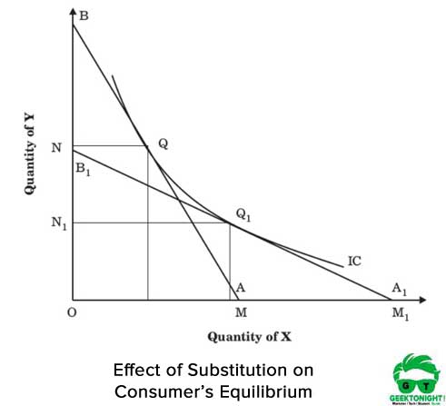
Line AB represents the original budget line. Q is the original point of consumer’s equilibrium, where AB is tangent to IC. At Q, the consumer purchases OM quantity of commodity X and ON quantity of commodity Y. If the price of commodity Y increases and the price of commodity X decreases, the new budget line would shift to B1A1. This new budget line is tangent to IC at Q1.

Therefore, the new equilibrium position of the consumer changes to Q1 from Q when the price of a commodity changes. At Q1, the consumer cuts down the units of commodity Y from ON to ON1 and purchases more units of X, OM to OM1.

However, the indifference curve remains the same. This movement along the indifference curve from Q to Q1 is known as the substitution effect.

Also Read: Utility in Economics

Price Effect on Consumer Equilibrium

As discussed above in the substitution effect, the prices of both the commodities change (Py increases and Px decreases). However, while considering the effect of price on consumer equilibrium, the price of only one commodity changes.

Therefore, the price effect is the change in the price of any one of the commodities due to which the quantity of commodities or services purchased changes.

Assume that the consumer purchases two commodities, X and Y. The price of commodity X decreases while the price of commodity Y and consumer’s money income remains constant. Let us understand this with the help of Figure 4.

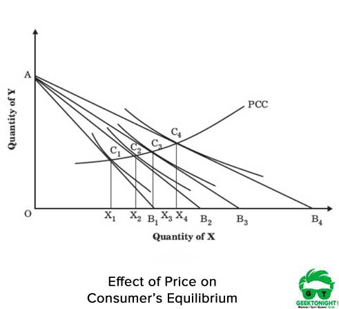
In Figure 4.14, the drop in the price of commodity X is denoted by the corresponding shifts of budget line from AB1 to AB2, AB2 to AB3 and AB3 to AB4. C1, C2, C3, and C4 represent a shift in consumer’s equilibrium. As the price of commodity X decreases, the consumer’s real income increases.

As a result, the consumer is able to purchase more units of both commodities X and Y. The curve PCC represents the Price Consumption Curve, which can be obtained by joining all equilibrium points C1, C2, C3, and C4.

Also Read: What is Market Equilibrium

Business Economics Tutorial

(Click on Topic to Read)

Go On, Share article with Friends

Did we miss something in Business Economics Tutorial? Come on! Tell us what you think about our article on Consumer Equilibrium | Business Economics in the comments section.