
Binomial Distribution
The binomial distribution is based on the concept of the Bernoulli trial. A Bernoulli trial is an experiment where only two outcomes are possible. A random variable X shall have a Bernoulli (P) distribution if:
X = 1 with probability p
X = 0 with probability1− p
Where 0 ≤ p ≤ 1.
Value X = 1 is often labelled a success and value X = 0 is termed a failure.
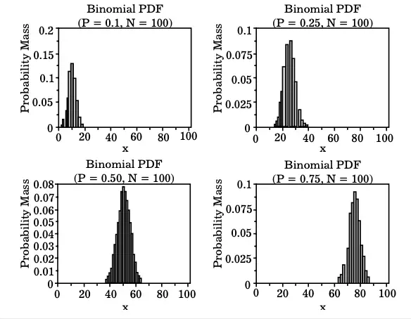
The binomial distribution is generally used to determine the probability of observing a required number (x) of successes in an experiment with N number of trials. The probability of success in a single trial is denoted by p. An assumption is made that binomial distribution p is fixed for all trials. The formula for the binomial probability mass function is as follows:
The plot of the binomial PDF for four values of p, i.e. 0.1, 0.25, 0.50, 0.75, and n = 100
Poisson Distribution
Poisson distribution was formulated by French mathematician Simon Denis Poisson. A Poisson random variable is the number of successes resulting from a Poisson experiment. Poisson distribution is the probability distribution of a random variable that results from a Poisson experiment. A Poisson experiment is a statistical experiment with the following attributes:
- The outcomes of the experiment are classified as successes or failures.
- The average number of successes in a particular area is denoted by μ and it is known.
- The probability of success in an event is proportional to the size of the region.
- The probability of success in an event in an extremely small region is almost zero.
A specified region could take many forms such as length, area, volume, period of time, etc.
The following notations are used frequently in a Poisson distribution:
- e: It is a constant that is approximately equal to 2.71828. In fact, e is the base of the natural logarithm system.
- μ: It is the average number of successes occurring in a specified region.
- x: It is the exact number of successes occurring in a specified region.
- P (x; μ): It is the Poisson probability of exact x successes occurring in a Poisson experiment. Here the mean number of successes is μ
The formula used to calculate the Poisson probability, once the average number of successes (μ) in a specified region is available, is given as follows:
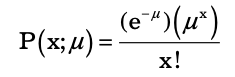
As mentioned earlier, here x is the actual number of successes resulting forming from the experiment, and e is approximately equal to 2.71828. A Poisson distribution has the following characteristics:
- The distribution mean is = μ.
- The variance is also = μ.
Normal Distribution
A normal equation describes a family of continuous probability distributions. It is used to present the real-valued random variables whose distributions are not known. The formula used in a normal distribution is as follows:
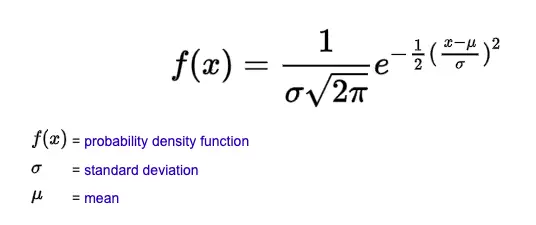
Here, μ is the mean of a normal distribution, x is a normal random variable, σ is the standard deviation of normal distribution, π = 3.14159, and e = 2.71828.
A normal distribution can be represented graphically and the two factors that affect the graph are the mean and the standard deviation. The location of the center of the graph is determined by the mean of the distribution, and the width and height of the graph are determined by the standard deviation.
The curve of the normal distribution is wide and short in the case of a large standard deviation. However, in the case of a small standard deviation, the normal distribution curve is narrow and tall. The curve of a normal distribution is bell-shaped and all normal distributions look symmetric.
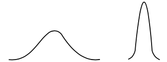
Normal Distribution Curves
In figure above, observe that the image on the left is shorter and wider as compared to the narrow and tall curve on the right. This is so because the curve on the right has a smaller standard deviation.
Let us discuss the relationship between probability and the normal curve. The continuous probability distribution nature of the normal distribution has multiple implications on probability.
The characteristics of normal distribution curves are as follows:
- The total area under the normal curve is 1.
- Mean, mode and median are all equal.
- The normal curve is symmetric around the mean, μ.
- All normal curves are symmetric about the mean μ, have a point of inflection at μ ± σ and are bell-shaped.
- For all values of x, all normal curves are positive. That is, f (x) > 0 for all x.
- The limit of f (x) as x approaches infinity is 0 and the limit of f (x) as x approaches negative infinity is also 0.
- The maximum height of any normal curve is at x = µ.
- The shape of a normal curve is dependent on its mean, i.e. μ, and its standard deviation σ.
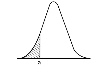
Normal Curve and α
With respect to the Figure above, the following points hold true:
- The area under the normal curve bound by α and infinity, that is, the non-shaded area gives the probability of X being greater than α.
- The area under the normal curve bounded by α and minus infinity, that is, the shaded area in the figure gives the probability of X being less than α.
Apart from the characteristics mentioned earlier, every normal curve (irrespective of the mean or standard deviation) conforms to the 68-95- 99.7 rule. It is a rule that is used in normal distributions to remember the percentage values that lie within a range of two, four, and six standard deviations around the mean. The precise values related to the rule are 68.27%, 95.45%, and 99.73%. According to this rule:
- 68% of the area under the normal curve falls within two standard deviations of the mean (x ± 1α).
- About 95% of the area under the normal curve falls within four-standard deviations of the mean (x ± 2α).
- About 99.7% of the area under the normal curve falls within six-standard deviations of the mean (x ± 3α.
A standard normal distribution has a mean of 1 and a standard deviation of 1. A standard normal distribution along with the 68-95-99.7 rule is depicted.
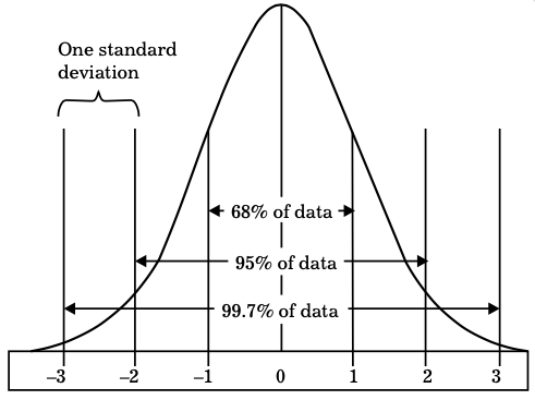
Standard Normal Distribution and the 68-95-99.7 Rule
Business Ethics
(Click on Topic to Read)
- What is Ethics?
- What is Business Ethics?
- Values, Norms, Beliefs and Standards in Business Ethics
- Indian Ethos in Management
- Ethical Issues in Marketing
- Ethical Issues in HRM
- Ethical Issues in IT
- Ethical Issues in Production and Operations Management
- Ethical Issues in Finance and Accounting
- What is Corporate Governance?
- What is Ownership Concentration?
- What is Ownership Composition?
- Types of Companies in India
- Internal Corporate Governance
- External Corporate Governance
- Corporate Governance in India
- What is Enterprise Risk Management (ERM)?
- What is Assessment of Risk?
- What is Risk Register?
- Risk Management Committee
Corporate social responsibility (CSR)
Lean Six Sigma
- Project Decomposition in Six Sigma
- Critical to Quality (CTQ) Six Sigma
- Process Mapping Six Sigma
- Flowchart and SIPOC
- Gage Repeatability and Reproducibility
- Statistical Diagram
- Lean Techniques for Optimisation Flow
- Failure Modes and Effects Analysis (FMEA)
- What is Process Audits?
- Six Sigma Implementation at Ford
- IBM Uses Six Sigma to Drive Behaviour Change
Research Methodology
Management
Operations Research
Operation Management
- What is Strategy?
- What is Operations Strategy?
- Operations Competitive Dimensions
- Operations Strategy Formulation Process
- What is Strategic Fit?
- Strategic Design Process
- Focused Operations Strategy
- Corporate Level Strategy
- Expansion Strategies
- Stability Strategies
- Retrenchment Strategies
- Competitive Advantage
- Strategic Choice and Strategic Alternatives
- What is Production Process?
- What is Process Technology?
- What is Process Improvement?
- Strategic Capacity Management
- Production and Logistics Strategy
- Taxonomy of Supply Chain Strategies
- Factors Considered in Supply Chain Planning
- Operational and Strategic Issues in Global Logistics
- Logistics Outsourcing Strategy
- What is Supply Chain Mapping?
- Supply Chain Process Restructuring
- Points of Differentiation
- Re-engineering Improvement in SCM
- What is Supply Chain Drivers?
- Supply Chain Operations Reference (SCOR) Model
- Customer Service and Cost Trade Off
- Internal and External Performance Measures
- Linking Supply Chain and Business Performance
- Netflix’s Niche Focused Strategy
- Disney and Pixar Merger
- Process Planning at Mcdonald’s
Service Operations Management
Procurement Management
- What is Procurement Management?
- Procurement Negotiation
- Types of Requisition
- RFX in Procurement
- What is Purchasing Cycle?
- Vendor Managed Inventory
- Internal Conflict During Purchasing Operation
- Spend Analysis in Procurement
- Sourcing in Procurement
- Supplier Evaluation and Selection in Procurement
- Blacklisting of Suppliers in Procurement
- Total Cost of Ownership in Procurement
- Incoterms in Procurement
- Documents Used in International Procurement
- Transportation and Logistics Strategy
- What is Capital Equipment?
- Procurement Process of Capital Equipment
- Acquisition of Technology in Procurement
- What is E-Procurement?
- E-marketplace and Online Catalogues
- Fixed Price and Cost Reimbursement Contracts
- Contract Cancellation in Procurement
- Ethics in Procurement
- Legal Aspects of Procurement
- Global Sourcing in Procurement
- Intermediaries and Countertrade in Procurement
Strategic Management
- What is Strategic Management?
- What is Value Chain Analysis?
- Mission Statement
- Business Level Strategy
- What is SWOT Analysis?
- What is Competitive Advantage?
- What is Vision?
- What is Ansoff Matrix?
- Prahalad and Gary Hammel
- Strategic Management In Global Environment
- Competitor Analysis Framework
- Competitive Rivalry Analysis
- Competitive Dynamics
- What is Competitive Rivalry?
- Five Competitive Forces That Shape Strategy
- What is PESTLE Analysis?
- Fragmentation and Consolidation Of Industries
- What is Technology Life Cycle?
- What is Diversification Strategy?
- What is Corporate Restructuring Strategy?
- Resources and Capabilities of Organization
- Role of Leaders In Functional-Level Strategic Management
- Functional Structure In Functional Level Strategy Formulation
- Information And Control System
- What is Strategy Gap Analysis?
- Issues In Strategy Implementation
- Matrix Organizational Structure
- What is Strategic Management Process?
Supply Chain

